
8.3.6 Application Example 8.11: Three-Phase Transformer with DC Bias Current
The losses of a 4.5 kVA three-phase transformer bank supplying power to resistive load under various DC bias conditions are to be measured. The measuring circuit for the Δ–Y0 connected three-phase transformer bank (see Appendix 4.2) is shown in Fig. 8.16. The transformer is operated at 75% of rated load with various (magnetizing current ranging from 0 to Im = 1.25 A) balanced DC bias currents injected on the Y0 side, and the DC copper, AC copper, and iron-core losses are to be measured separately. Such DC currents can be generated by either unbalanced rectifiers, geomagnetic storms [31,80,93,94], or nuclear explosions.
Solution to Application Example 8.11
Measured iron-core and copper losses vary with the DC bias current and are listed in Table E8.11,1a, Table E8.11,1b and Table E8.11,1ac [94].
Table E8.11.1a
Measured Iron-Core and Copper Losses of 4.5 kVA Δ-Y0 Connected Transformer with DC Bias for a Rated Line-to-Line Input Voltage of 242 V [94]
| DC bias current (A) | Iron-core losses (W) | AC copper losses (W) | DC copper losses (W) | Total losses (W) | Output power (W) |
| 0.00 | 72.2 | 78.1 | 0.0 | 150.3 | 3340 |
| 0.56 | 79.9 | 78.9 | 0.4 | 159.2 | 3327 |
| 0.74 | 83.1 | 79.1 | 0.7 | 162.9 | 3316 |
| 1.01 | 88.7 | 81.8 | 1.3 | 171.8 | 3306 |
| 1.25 | 101.7 | 85.2 | 1.9 | 188.7 | 3293 |

Table E8.11.1b
Measured Iron-Core and Copper Losses of 4.5 kVA Δ-Y0 Connected Transformer with DC Bias for a Below-Rated Line-to-Line Input Voltage of 230 V [94]
| DC bias current (A) | Iron-core losses (W) | AC copper losses (W) | DC copper losses (W) | Total losses (W) | Output power (W) |
| 0.00 | 62.9 | 67.9 | 0.0 | 130.8 | 2958 |
| 0.55 | 68.6 | 69.3 | 0.4 | 138.3 | 2950 |
| 0.76 | 72.0 | 72.1 | 0.7 | 144.8 | 2944 |
| 1.03 | 90.7 | 72.3 | 1.3 | 164.3 | 2940 |
| 1.24 | 95.1 | 76.2 | 1.9 | 173.2 | 2925 |

Table E8.11.1c
Measured Iron-Core and Copper Losses of 4.5 kVA Δ-Y0 Connected Transformer with DC Bias for an AboveRated Line-to-Line Input Voltage of 254 V [94]
| DC bias current (A) | Iron-core losses (W) | AC copper losses (W) | DC copper losses (W) | Total losses (W) | Output power (W) |
| 0.00 | 82.5 | 87.0 | 0.0 | 169.5 | 3663 |
| 0.56 | 88.4 | 86.7 | 0.4 | 175.5 | 3657 |
| 0.74 | 93.9 | 87.4 | 0.7 | 182.0 | 3658 |
| 1.02 | 103.0 | 90.0 | 1.7 | 194.3 | 3654 |
| 1.25 | 109.8 | 93.5 | 1.9 | 205.3 | 3645 |

Table E8.11,1a, Table E8.11,1b and Table E8.11,1ac demonstrate that the DC copper loss due to the DC bias current is negligibly small. However, the AC copper losses and the iron-core losses increase at rated input voltage (240 V) by about 10% and 40%, respectively, due to a DC bias current of 100% of the magnetizing current magnitude (Im = 1.25 A) within the Y0 connected windings; thus the efficiency of the transformer decreases from

8.3.7 Discussion of Results and Conclusions
New approaches for the real-time monitoring of three-phase transformer power loss have been described and applied under nonsinusoidal operation. Accurate (maximum error of 0.5 to 15%), inexpensive ($3,000 for PC and A/D converter) computer-aided monitoring circuits have been devised and their applications demonstrated.
The digital version of the proposed measuring circuits has the following advantages as compared with the analog circuit of Arri et al. [90]:
a) Measuring circuits are suitable for three-phase transformers with various commonly used connections (any combination of Y ungrounded, Y grounded, and Δ connections). Because the iron-core and copper losses of grounded three-phase transformers can be correctly measured, the method is also applicable for loss monitoring of power transformers under DC bias that can be generated by either unbalanced rectifiers, geomagnetic storms [31,80,93,94], or nuclear explosions.
b) Fewer current and voltage transformers are used (only four CTs and five PTs are required, as shown in Fig. 8.20, comparing to nine CTs and nine PTs used in [90]), and therefore, the measurement accuracy is higher.
c) The software [70] of this monitoring approach does not rely on the discrete Fourier transform (DFT) but on a more accurate transform, which is based on functional derivatives and can also be computed via the fast Fourier transform (FFT). With such online monitoring, the iron-core and copper losses can be sampled within a fraction of a second. Moreover, current and voltage wave shapes, harmonic components, total harmonic distortions, input, output, apparent powers, and the efficiency can be dynamically displayed and updated, and it is quite straightforward to measure the transformer derating under various nonsinusoidal operations [73]. The software is compatible with some commercially available data-acquisition tools [95–101].
Online measurement of power transformer losses has the following practical applications: apparent power derating, loading guide, prefault recognition, predictive maintenance, and transformer aging and remaining life quantification. The method proposed in this section can be used as a powerful monitoring tool in these applications. The method is suitable for any kind of transformer regardless of size, rating, type, different magnetic circuit (core or shell, three or five limbs), cooling system, power system topology (nonsinusoidal and unbalanced), etc.
8.3.8 Uncertainty Analysis [102]
The standard ANSI/NCSL Z540-2-1997 (R2002) recommends that the maximum error analysis as used in Section 8.3.3 be replaced by the expression of uncertainty in measurement. The rationale is that the growing international cooperation and the National Conference of Standards Laboratories International (NCSLI) have recommended that standard. The standard ANSI/NCSL Z540-2-1997 (R2002) “is an adoption of the International Organization for Standardization (ISO) Guide to the Expression of Uncertainty in Measurement to promote consistent international methods in the expression of measurement uncertainty within U.S. standardization, calibration, laboratory accreditation, and metrology services.” This standard serves the following purposes:
1. It makes the comparison of measurements more reliable than the maximum error method.
2. Even when all of the known or suspected components of error have been evaluated and appropriate corrections have been applied there still remains an uncertainty about the correctness of the stated result.
3. The evaluation and expression of uncertainty should be universal and the method should be applicable to all kinds of measurements.
4. The expression of uncertainty must be internally consistent and transferable.
5. The approach of this standard has been approved by the Bureau International des Poids et Mesures (BIPM).
It is for these reasons that the measurement errors in [74] have been expressed by the uncertainty as recommended by the standard.
8.3.9 SCADA and National Instrument LabVIEW Software [103]
Supervisory control and data acquisition (SCADA) plays an important role in distribution system components such as substations. There are many parts of a working SCADA system, which usually includes signal hardware (input and output), controllers, networks, human–machine interface (HMI), communications equipment, and software. The term SCADA refers to the entire central system, which monitors data from various sensors that are either in close proximity or off site. Remote terminal units (RTUs) consist of programmable logic controllers (PLCs). RTUs are designed for specific requirements but they permit human intervention; for example, in a factory, the RTU might control the setting of a conveyer belt, but the speed can be changed or overridden at any time by human intervention. Any changes or errors are usually automatically logged and/or displayed. Most often, a SCADA system will monitor and make slight changes to function optimally and they are closed-loop systems and monitor an entire system in real time. This requires
• data acquisitions including meter reading,
• checking the status of sensors, the data of which are transmitted at regular intervals depending on the system. Besides the data being used by the RTU, it is also displayed to a human who is able to interface with the system to override settings or make changes when necessary.
8.4 Tools for improving reliability and security
SCADA equipment such as RTUs and PLCs are applications of telecommunications principles. Interdisciplinary telecommunications programs (ITPs) [104] combine state-of-the-art technology skills with the business, economic, and regulatory insights necessary to thrive in a world of increasingly ubiquitous communications networks. ITPs are served by faculties in economics, electrical engineering, computer science, law, business, telecommunications industry, and government. They address research in wireless, cyber-security, network protocols, telecom economics and strategy, current national policy debates, multimedia, and so forth. Key topics by ITPs are
• Security and reliability of utility systems addressing a range of security-related issues on physical and information security as well as vulnerability assessment and management. The major areas discussed include physical security and access control, asset protection, information systems analysis and protection, vulnerability, assessment, risk management, redundancy, review of existing security and reliability in power systems, new security guidelines, threat response plan, and contingency operation.
• Risk analysis and public safety review various kinds of risks ranging from floods, power outages, and shock to biological hazards. Various approaches to setting safety standards and minimizing risks are explored.
• Current, future, and basic technical concepts of telecommunications systems are studied. They include an in-depth look at basic telecom terminology and concepts, introductions to voice and data networks, signaling, modulation/multiplexing, frequency-band and propagation characteristics, spectral analysis of signals, modulation (amplitude modulation AM, frequency modulation FM, phase modulation PM, and pulsecode modulation PCM), digital coding, modulation multiplexing, detection, transmission systems, and switching systems with an introduction to different network configurations and traffic analysis.
• Data communications define data and computer communications terminology, standards, network models, routing and switching technologies, and communication and network protocols that apply to wide-area networks WANs, metropolitan-area networks MANs, community wireless networks CWNs, and local-area networks LANs. Studies therefore focus on asynchronous and synchronous wide-area networks such as frame relay and synchronous optical networks SONETs, the Internet, routers, selected Internet applications, and Ethernets.
• Applied network security examines the critical aspects of network security. A technical discussion of threats, vulnerabilities, detection, and prevention is presented. Issues addressed are cryptography, firewalls, network protocols, intrusion detection, security architecture, security policy, forensic investigation, privacy, and the law.
• The emerging technology of internet access via the distribution system is addressed [105].
The 2003 U.S.–Canada blackout is analyzed in [106] and recommendations are given for prevention of similar failures in the future. Reliability questions are addressed in [1,107]. With the advent of distributed generation [108,109], the control of power systems will become more complicated due to the limited short-circuit capability of renewable sources and their nonsinusoidal voltage and current wave shapes [110].
8.4.1 Fast Interrupting Switches and Fault-Current Limiters
Fast interrupting switches and fault-current limiters serve to maintain the stability of an interconnected system by isolating the faulty portion or by mitigating the effect of a fault on the healthy part of the power system. Fast interrupting switches are used to prevent ferroresonance due to the not quite simultaneous closing of the three phases, and to ease reclosing applications. In the first application the almost simultaneous switching of the three phases prevents the current flows through the capacitance of a cable, which is required for inducing ferroresonant currents (see Chapter 2), whereas in the latter the reclosing should occur within a few cycles as indicated in Chapter 4.
Fast Interrupting Switches (FIS)
Fast interrupting switches [111] rely on sulfur hexafluoride (SF6) as a quenching medium resulting in an increased interrupting capability of the circuit breaker. SF6 is an inorganic compound; it is a colorless, odorless, nontoxic, and nonflammable gas. SF6 has an extremely great influence on global warming and therefore its use should be minimized or entirely avoided. From an environmental point of view a circuit breaker is expected to use smaller amounts of SF6 or to adopt as a quenching medium a gas that causes no greenhouse effect. Research is performed to substitute SF6 by a greenhouse benign alternative quenching gas. The series connection of an FIS with a fault-current limiter either reduces the interrupting conditions or makes the substitution of SF6 with a less effective quenching gas possible. For this reason it is important to investigate the dependence of the interrupting condition on the circuit parameters as will be done in the next section.
Fault-Current Limiters (FCLs)
Fault-current limiters are installed in transmission and distribution systems to reduce the magnitude of the fault current and thereby mitigate the effect of the fault on the remaining healthy network. The fault-current limiter is a device having variable impedance, connected in series with a circuit breaker (CB) to limit the current under fault conditions. Several concepts for designing FCLs have been proposed: some are based on superconductors [112–114], power electronics components [115–118], polymer resistors [119], and control techniques based on conventional components [120]. FLCs not only limit the fault currents but can have the following additional functions:
• reduction of voltage sags during short-circuits [121],
• improvement of power system stability [122,123],
• reduction of the maximum occurring mechanical and electrical torques of a generator [124], and
• easement of the interrupting burden on circuit breakers by limiting the fault current to a desirable level.
Note that in the latter case the burden on the circuit breaker depends not only on the interrupting current but also on the transient recovery voltage (TRV) appearing across the contacts of a circuit breaker. It is conceivable that a limiting impedance of the FCL and a stray capacitance can result in a change of the TRV and may bring about a more severe interrupting duty than in the absence of an FLC. In the following section the influence of a resistive and an inductive FLC on the interrupting duty of a circuit breaker will be investigated for various fault locations. First, a fault occurring near an FCL must be addressed because it produces the maximum fault current that a circuit breaker must interrupt. In this case the TRV across the circuit breaker will be not as severe as compared with the case where the fault occurs a few kilometers from the terminals of the FCL. However, a fault a few kilometers from the FCL must also be taken into account because the rate of rise of the recovery voltage (rrrv) is higher in this case than for a fault occurring near the FCL.
8.4.2 Application Example 8.12: Insertion of a Fault Current Limiter (FCL) in the Power System
The system voltage and frequency of a transmission system are assumed to be VL–L = 275 kV (or VL–N = 159 kV) and 60 Hz, respectively. A symmetrical three-phase to ground short-circuit is assumed to occur at a distance ℓ of 0 to 8 km from the load-side terminals of the FCL. Figure E8.12.1 shows the corresponding single-phase equivalent circuit; on the supply-side the inductance Ls = 6.69 mH and the capacitor Cs = 750 nF are given. At a fault near the circuit breaker (CB)—in the absence of an FCL—the CB is assumed to interrupt 63 kArms at a rate of rise of the recovery voltage (rrrv) of 2.3 kV/μs. In the absence of an FCL the current at a distance ℓ of 1 km, 4 km, and 8 km is 90%, 68%, and 51% of 63 kArms. CFCL = 1 nF represents the stray capacitance to ground of the FCL, and the transmission line inductance Ltr and capacitance Ctr per unit length are 0.8 mH/km and 15 nF/km, respectively. The current interruption process of the circuit breaker can be assumed to be that of an ideal switch. Design the ZFCL = RFCL + jωLFCL and estimate the stray capacitance Cstray connected in parallel with LFCL.

Solution to Application Example 8.12
It is assumed that the FCL produces a limiting impedance ZFCL of either a resistive type or an inductive type as is illustrated in Fig. E8.12.2. The resistance RFCL is in the range of 1 to 9 Ω and the inductance LFCL in the range of 2.6 to 23.9 mH; that is, for 60 Hz the resistive (RFCL) and reactive (2πf · LFCL) components are about the same. In the latter case the capacitance Cstray (10 to 100 nF) represents a stray capacitance and is connected in parallel with LFCL.

8.4.3 Intentional Islanding, Interconnected, Redundant, and Self-Healing Power Systems
The present interconnected power system evolved after 1940 and represents an efficient however complicated energy generation, distribution, and utilization network. It is reliable but also vulnerable to sabotage, economic issues, distributed generation, and regulations as well as a lack of appropriately trained or educated engineers. Power systems can be configured in multiple ways: at one extreme we have one large power source that delivers all the required power to multiple loads over transmission lines of varying lengths. At the other extreme there are individual sources that supply the needs for each and every load. In between we have multiple sources (e.g., distributed generation) and loads of varying size that are connected by many transmission lines to supply the loads. The fundamental issue is how to balance efficiency, reliability, and security. For relatively small systems a single source serving multiple loads that are distributed over relatively small distances has the advantages of being able to share capacity as the demand varies from load to load as a function of time and to take advantage of the efficiencies of size. A single source for either one single load or several loads is the easiest to control (e.g., isochronous control) and, in many respects, the most secure, as possible failure mechanisms are associated with one source only. By connecting given loads to multiple sources (e.g., with drooping frequency-load characteristics, see Problems 4.12 to 4.14 of Chapter 4) with multiple transmission lines we increase the reliability, as the failure of any one source or transmission line can be compensated for by picking up the load from other sources or over other transmission lines. However, as the number of lines and sources becomes large the control problem becomes too large to be managed centrally. This problem of distributed control for complicated power networks is closely related to the same problem in communications, biological, economic, political, and many other systems.
In the case of distributed generation with renewable energy sources (e.g., wind, solar) additional constraints enter the control approach where the renewable sources are operated at near 100% capacity by imposing droop characteristics with steep slopes. The intermittent operation of renewable sources requires that peak-power plants are able to take over when the renewable sources are unable to generate power. In order to minimize peak-power generation (e.g., spinning reserve) capacity it will be advisable to also rely on energy storage plants (e.g., hydro, compressed air, supercapacitors).
In the following we explore the requirements necessary so that power systems can organize themselves. The information that is required to operate a conventional stand-alone power plant with isochronous control is relatively well known. However, it is much less clear what information one needs to operate a network that is faced with new and changing requirements and constraints that are brought about by new security problems, environmental regulations, distributed generation, competition, etc. Questions to be addressed by the control and dispatch center of a power system include the following: capacity at which each transmission line and power plant is operating, fuel reserves, frequency and phase of the generators, weather forecast, scheduled and nonscheduled power exchanges, times to shed non-critical loads or pick up new loads, repair times for various kinds of damage and maintenance, hierarchy of controls, and design of the system so that if a terrorist has access to a port on the network the damage he can do is limited. How does the probability that this can happen increase with the number of ports/buses on the network? It is advisable to look at the design of other complex systems that organize themselves as possible models for our power system. Systems that can be considered as role models include the Internet, multistream multiprocessor computer systems for parallel computing, and biological systems.
The systems with the most closely related set of constraints to the problem of the allocation of generation capacity and the distribution of power for varying loads with the loss of a generator or a transmission line are communications networks. These networks have a large number of sources and sinks for information that may be connected by many transmission or communication lines. Strategies for the design of these networks that take into account the cutting of communication lines or the loss of nodes such as telephone switches have been developed [125]. Typical designs for reliability include dual rings and meshes. Considerable savings can be obtained as well as an increase in reliability by the use of meshes. In order for these networks to be effective under varying levels and patterns of use, each node needs information about the traffic flow and the state of adjacent nodes on the network. If the proper information on the bandwidth and traffic are updated on a continuing basis, then the nodes can be prepared to allocate the traffic around a given fault when it occurs. Thus a given node can know at all times how it will reroute the traffic if a communication line is broken or an adjacent node is lost. This can be done without a central command system and in a sense provides a self-organizing system to correct for communication line outages or the loss of a node. Strategies used in communication theory can be effectively employed or modified to improve the reliability of power systems and their efficient operation.
Biological systems can serve as a role model for the design of power systems. Biological systems are highly adaptive and provide both repair and controls that allow them to deal with a large number of unexpected events. These systems use a hierarchy of control systems to coordinate a large number of processes. The brain typically controls the action of the body as a whole, but individual components such as the heart have local control systems that respond to demand for oxygen as communicated to it by signals from other sensory systems such as the baroreceptors. Thus there are functions that require a global response and there are others that are better dealt with locally. Additionally, different biological control systems respond with different time constants [126]. Similarly, power systems have parameters such as fuel reserves with relatively long time constants and other events such as transmission line short-circuits that need to be responded to in fractions of seconds or minutes.
Neural networks are useful ways to approach many complex pattern recognition and control problems that are at least philosophically modeled on biological systems, which use both feedback and feed-forward networks to generate adaptive responses to problems. One of the most common neural networks adjusts the connection weights, using a back propagation algorithm to adapt the network to recognize the desired pattern. This property can be used to develop a control system that has the best response to a wide variety of network problems. Feed-forward networks can be used to anticipate the power system behavior and to prevent problems such as a cascade of network overloads. Power system control and security problems can be formulated in such a way that neural networks can be used as portions of an effective control system. It is to be noted that we can now place computers in the feedback loop of a control system to perform much more complex functions than the classical control systems with a few passive elements.
The three power systems (Western, Eastern, and Texan) within the contiguous United States and their DC links operate quite effectively and reliably. This is so because there is distributed control within the transmission system and the distribution feeders: the integrity of the three power systems – including the DC link between the three grids – is maintained through relaying and supervisory control. The everyday operation of power systems takes into account single power plant and single transmission line outages; contingency plans are readily available for the operators. The question arises: what must be done if major emergencies happen? We can identify four types of emergencies:
1. Failure of a major power system component (e.g., power plant, transmission line).
2. Simultaneous failure of more than one major component at different locations such as caused by terrorist attacks.
3. Outage of a power system within an entire region caused by a nuclear explosion or geomagnetically induced currents (GICs) [127].
4. Disruption of the sensing or communication network.
Although the first type of failure can be handled by the present expertise or equipment of power system operators by established contingency plans, the last three failure modes are not planned for because they do not commonly occur. Strategies and countermeasures must be devised so that the power system will be able to survive such major emergencies.
8.4.4 Definition of Problem
The problem at hand is multifaceted: it involves behavior, chemical, biological, economic, and engineering sciences. Although interdisciplinary in its nature, only topics involving electrical, telecommunications, and civil or architectural engineering will be addressed.
These sciences will be employed to discuss the following:
1. What can be done to prepare the power system prior to an emergency?
2. What should be done during the failure?
3. What will be done after the failure has occurred?
4. What strategies for efficiency improvements and maintaining regulatory constraints must be addressed?
5. What educational aspects must be highlighted at the undergraduate and graduate levels?
These queries will now be addressed in detail.
8.4.5 Solution Approach
There are several approaches for the control of the power networks. The first one draws on the techniques that have been used to control communications networks, that is, to provide each power source with the intelligence to keep track of its local environment and maintain the plans on how it would reroute power if a transmission line is cut or if an adjacent node is either dropped out of the network or has a sudden change in load. This leads to an examination of the power distribution networks to see how the network can be configured to increase its reliability, and this may well mean adding some new transmission lines that enable loads to be supplied from multiple sources. In addition it will require multiple communication links between critical loads and generating power plants. A result of this approach is to allow local nodes on the network to have a high degree of independence that lets them control themselves. This gives both the loads and the generators great flexibility. Writing the rules so that such a system is stable, economical, reliable, and secure is major.
A second approach uses biological systems as a model to develop a hierarchy of controls and information processing that will improve the overall efficiency and reliability of the system. The objective of this effort is the separation of the control problems so that the control of each function is handled by a network that functions as efficiently as possible. This means handling local problems locally and scaling up to larger regions only when it leads to improved system performance in terms of efficiency, reliability, and security. It also means finding a way to make the control system respond on the time scale needed to handle the problem; that is, there are multiple control systems that interface and transmit information between them. Biological systems are often extremely good at optimizing the distribution of controls and efficiency; they are a good starting point to look for ideas for solving related problems. For example, sharks and rays can detect electric fields as small as 10–7 V/m using a combination of antennas, gain, and parallel processing to detect fish and navigate with signals that at first glance are below the noise level. The way humans use past experience to anticipate future problems may well provide us with an approach to using neural networks as a part of the control system and preventing terrorist attacks.
What Can Be Done to Prepare the Power System Prior to an Emergency? This is the most important part for coping with emergencies where several power plants or transmission lines fail or where the power system of an entire region is affected. It is recommended to divide each of the three power pools into independently operating power regions (IOPRs), with distributed intelligence so that in the case of a major emergency – where short-circuits occur – fault-current limiters (FCLs) separate [121–124] within a fraction of a 60 Hz cycle the healthy grid from the faulty section. Each of the designated IOPRs must be able to operate independently and maintain frequency and voltage at about their nominal values either with isochronous or drooping frequency-load control. To achieve this, optimal reconfiguration of the power system must occur within milliseconds permitting intentional islanding operation. If necessary, optimal load shedding must take place but maintaining power to essential loads. To ease such an optimal reconfiguration, provisions must be made to relax usually strict requirements such as voltage and power quality constraints. The ability to communicate and to limit short-circuit currents within milliseconds will be an essential feature of this strategy. It is well known that nuclear explosions generate plasma that is similar to that of solar flares and therefore induce low frequency or quasi-DC currents within the high-voltage transmission system. To minimize the impact of nuclear explosions on the transmission system, three-limb, three-phase transformers with small zero-sequence impedances Z0 will have to be used [31,80,94,127] and DC current compensation networks [94] will have to be installed at key transformers connected to long transmission lines to enforce balanced DC and AC currents.
What Should Be Done during the Failure? In an emergency the fault current limiters sense overcurrents and limit these. Thereafter, reclosing switches connected in series with the FCLs will attempt to restore the connection within a few 60 Hz cycles. If the fault duration is longer than a few 60 Hz cycles then circuit breakers connected in series with the FCLs (see Fig. 8.21) will permanently open the faulty line until the source of the fault has been diagnosed. Reclosing switches are employed first because a great number of faults are temporary in their nature. This even applies to a nuclear explosion that lasts only a few seconds but generates plasma that exists for about 60 s. This plasma consists of charged particles that radiate electromagnetic waves and therefore induce low-frequency or quasi-DC currents in the long high-voltage transmission lines. If these quasi-DC currents are balanced within the three phases, the reactive power demand and its associated voltage drops are manageable if the zero-sequence impedance Z0 of three-limb, three-phase transformers is small. For unbalanced DC currents the reactive power demand and its associated voltage drops are large. For this reason a temporary (seconds) interruption of transmission lines might be beneficial until the plasma has dispersed. This is analogous to a patient who will be rendered unconscious while the operation progresses. Instead of enforcing an interruption another possibility is to enforce a balance of the quasi-DC currents with DC current compensation networks [94].

What Will Be Done after the Failure Has Occurred? It is essential that the IOPRs can operate for a longer period of time (e.g., days) so that essential loads can be supplied. If there is a problem with maintaining frequency and voltage control then optimal load shedding will take place. The protocol for optimal load shedding must be defined before an emergency occurs. Relying on a central clock (e.g., National Institute of Standards and Technology, NIST), the paralleling of individual IOPRs can proceed to restore the integrity of each of the three power systems within the US. An alternate strategy is to have a number of atomic clocks located throughout the networks that can provide both the frequency and phase information.
What Strategies for Efficiency Improvements and Maintaining Regulatory Constraints Must Be Addressed? Efficiency improvement and maintaining power quality and other regulatory constraints will be unimportant while the failure occurs. For all other times an algorithm developed operates the power system efficiently for given constraints. The development of such software combines harmonic load flow [78], power quality [32,110,128–130] constraints, capacitor switching, and optimization where efficiency and cost are components of the objective function [131–134].
Reliability
Most short-circuits in power systems occur because of insulation failure. The breakdown of the insulation depends on the voltage stress integrated over time. Although the time component cannot be influenced, the voltage stress across a dielectric can be reduced. With improved semiconductor technology and variable-frequency drives (VFDs) based on pulse-width modulation (PWM), the induction motor has become a viable alternative – as compared with DC motor drives – for many applications. The majority of these applications are usually under the 2 kV and the 1 MW range. Even with advancements in technology, the induction, synchronous, or permanent-magnet motors or generators experience failures of their windings due to large voltage stress when fed by PWM frequency current- or voltage-source converters. Repair work and fault analysis and research show that the majority of insulation failures occur near the last turn of the first coil prior to entering the second coil of the windings. Wave-propagation theory shows that forward- and backward-traveling waves superimpose so that the maximum voltage stress does not necessarily occur at the terminals of a winding but somewhere in between the two terminals. Because of the repetitive nature of PWM pulses the damping due to losses in the winding and iron core cannot be neglected. Work by Gupta [135–137] and many others [138–154] neglect the damping of the traveling waves; therefore it cannot predict the maximum voltage stress of the winding insulation. Figure E3.14.1 of Chapter 3 illustrates a part of a machine winding that can be modeled by inductances and capacitances – a model suitable for the traveling wave theory. This model neglecting losses has been used in [135]. By computing and measuring the maximum voltage stress as a function of PWM switching frequency and duty cycle, one finds that current-source inverters and lightning strikes generate the largest voltage stress because of their inherent current spikes resulting in a large L(di/dt).
Demand-Side Management Programs
In the upcoming years, utilities continue to face fundamental changes:
• Greater access by utilities and others to the transmission systems of other utilities
• Competition for retail customers from other power sources, self-generation or cogeneration, and from other utility suppliers
• Reduction in the cost of renewable resources
• Growing use of demand-side management (DSM) programs as capacity and energy resources
• Increased concern with the environmental consequences of electricity production
• Growing public opposition to construction of new power plants
• Uncertainty about future load growth, fossil-fuel prices and availability, and possible additional regulations
The traditional approach to utility planning with its narrow focus on utility-built power plants is no longer adequate. A new paradigm for utility resource planning has been promoted [155]. The new approach should account for the availability of DSM and renewable-energy technologies and the public concern with environmental qualities.
Demand-side management programs present modest but growing sources of energy and capacity resources. In 1993, DSM programs cut annual electricity sales by 1.5% and potential peak demand by 6.8% [156,157]. DSM programs include a variety of technologies related to energy efficiency, load management, and fuel switching.
A survey of 2321 DSM programs conducted by 666 electric utilities in the United States indicated a wide range of technology alternatives, market implementation techniques, and incentive structures [158]. Of the total programs surveyed, 64% include residential customers, 50% commercial customers, 30% industrial customers, and 13% agricultural customers. Moreover, 56% of the programs emphasize peak-clipping goals and 54% feature energy-efficiency goals. Load-shifting, valley-filling, and load-growth objectives are also associated with reported DSM programs.
Load control programs are the most prevalent forms of demand-side management practiced by utilities interested in peak clipping. Three types of techniques are commonly used by utilities that would want to exercise control over customer loads:
• Direct control techniques by utilizing a communications system to remotely affect load operation. The communication technologies used include VHF radio, power liner carrier, ripple, FM-SCA radio, cable TV, and telephone.
• Local control techniques through the promotion and use of demand control equipment that operates according to local conditions. The technologies used in local control include temperature-activated cycling (mostly for the control of air conditioners), timer tripping (on pumps), and various mechanisms that employ timers, interlocks, and/or multiple function demand limiters.
• Distributed control techniques that merge both direct and local control concepts by using a communications system to interface with and/or activate a local control device.
In the EPRI survey [158], a total of 467 load control programs have been reported by 445 different U.S. utilities. The vast majority (440) of reported programs utilize direct control technologies. Only 19 programs employ local control technologies and 8 programs use distributed controls involving interfacing between direct and local control technologies.
A crucial part of any DSM program is electrical load monitoring. Most utilities rely on revenue meters at the point of electrical entrance service to individual buildings or group of buildings. Some DSM programs may require the installation of additional meters for individual electricity-consuming devices such as lighting systems, ventilation fans, or chillers. With these additional meters, controls of targeted equipment can be performed. To make implementation of DSM programs cost-effective, there is an increased interest in monitoring techniques that allow detection and separation of individual loads from measurements performed at a single point (such as the service entrance of a building) serving several electricity-consuming devices. Such techniques have been proposed and have been shown to work relatively well for residential buildings but have not been effective for commercial buildings with irregular and variable loads [159].
Electricity production, transmission, and distribution have substantial environmental costs. Utilities use different methods to assess these impacts [160]. The simplest approach ignores externalities and assumes that compliance with all government environmental regulations yields zero externalities. A more complicated approach consists of ranking and weighting the individual air, water, and terrestrial impacts of different resource options. Some utilities utilize approaches that require quantification (such as weight measured in ton-force of either sulfur dioxide or carbon dioxide emitted per million BTU of coal) and monetization (dollars of environmental damage per ton-force of either carbon dioxide or sulfur dioxide) of the emissions associated with resource options. However, since the estimates of monetized environmental costs vary so much, many utilities are reluctant to use these approaches to assess the environmental externalities of resource options.
Distribution circuits with high reliability indices (e.g., flower configuration) and the use of self-healing system configurations are more expensive than the radial, open-loop, and ring configurations. At present the distribution system contains not much intelligence if one ignores SCADA. In the future the subtransmission and distribution system will have to be equipped with intelligent components as well so that the distributed generation can play a role even if central power stations go off-line because of faults.
8.4.6 Voltage Regulation, Ride-Through Capabilities of Load Components; CBEMA, ITIC Tolerance Curves, and SEMI F47 Standard
Voltage Regulation VR
Faults (e.g., short-circuits), as discussed in Chapters 1 and 4, and environmental (e.g., lightning) events addressed in Chapters 1 and 4 cause the voltage to deviate from its rated wave shape (e.g., magnitude and waveform). The steady-state voltage deviation is measured by the voltage regulation [161]

where VR is the percent voltage regulation, which is 100% for |V| = Vrated. The voltages |V| and Vrated are the measured rms voltage and the rated (nominal) voltage, respectively. The voltage regulation is a measure for the strength of a bus, that is, the ability of the bus to supply current without changing its voltage amplitude. The short-circuit ratio (SCR = Isc/Irated) discussed in Chapters 1 and 4 is indicative of the strength of a power system. Renewable sources have a limited short-circuit current capability, and for this reason they lead to weak systems. Typical values of SCR are in the range from 20 to 200 for residential and 1000 or more for industrial circuits. Whereas the voltage regulation characterizes steady-state voltage amplitudes, the voltage-tolerance (also called power-acceptability and equipment-immunity) curves measure the change in bus voltage during a few 60 Hz cycles.
Voltage-Tolerance CBEMA and ITIC Curves
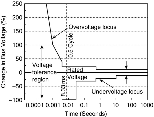
The voltage-tolerance curves [162–165] are loci drawn in the bus voltage versus duration time semilogarithmic plane. The loci indicate the tolerance of a load to withstand either low or high voltages of short duration (few 60 Hz cycles). Figure 8.22 illustrates the voltage-tolerance curve established by the Computer Business Equipment Manufacturers Association (CBEMA), usually called the CBEMA curve. There are two loci: the overvoltage locus above the rated voltage value and the undervoltage locus below the rated voltage value. The linear vertical axis (ordinate) of Fig. 8.22 represents the percent change in bus voltage from its rated value. The semilogarithmic horizontal (abscissa) axis indicates the duration of the voltage disturbance either expressed in 60 Hz cycles or seconds. The steady-state value of the undervoltage locus approaches −13% below the rated voltage. Overvoltages of very short duration are tolerable if the voltage values are below the upper locus of the voltage-tolerance curve. The term “voltage tolerance region” in Fig. 8.22 identifies the permissible magnitudes for transient voltage events. Voltage events are due to lightning strikes, capacitor switching, and line switching due to faults.

In 1996 the CBEMA curve was replaced by the ITIC curve of Fig. 8.23 as recommended by the Information Technology Industry Council (ITIC).
SEMI F47 Standard
The manufacturing process for semiconductor equipment is very sensitive to voltage sags. For this reason the semiconductor industry joined forces and established criteria for permissible sags that will not affect the manufacturing process. Figure 8.24 shows measured voltage sags that have been characterized by their magnitudes and durations and are plotted along with the equipment ride-through standard for semiconductor manufacturing equipment [166–169]. The circled data in Figure 8.24 represent events that resulted in the process interruption of semiconductor manufacturing. In comparison to the CBEMA and ITIC curves, the SEMI F47 curve addresses low-voltage conditions only.

8.4.7 Application Example 8.13: Ride-Through Capability of Computers and Semiconductor Manufacturing Equipment
Determine for the data given in Table E8.1.1 the ride-through capability of
• semiconductor manufacturing equipment.
Solution to Application Example 8.13
a) Ride-through capability based on the CBEMA or ITIC voltage-tolerance curves:
• 1 min at 90% of rated voltage: ride-through is possible,
• 1 s at 130% of rated voltage: ride-through is not possible,
• 0.1 s at 40% of rated voltage: ride-through is not possible,
• 0.1 s at 150% of rated voltage: ride-through is not possible,
• 0.01 s at 50% of rated voltage: ride-through is possible.
b) Ride-through capability based on SEMI F47 standard:
• 1 min at 90% of rated voltage: ride-through is possible (borderline),
• 1 s at 130% of rated voltage: ride-through is possible,
• 0.1 s at 40% of rated voltage: ride-through is not possible,
• 0.1 s at 150% of rated voltage: ride-through is possible,
• 0.01 s at 50% of rated voltage: ride-through is possible.
8.4.8 Backup, Emergency, or Standby Power Systems (Diesel-Generator Set, Batteries, Flywheels, Fuel Cells, and Supercapacitors)
Standard IEEE-446 [170] gives definitions related to emergency and standby power systems, general need guidelines, systems and hardware, maintenance, protection, grounding, and industry applications. An important variable – besides the voltage amplitude characterized by the voltage regulation VR – for the safe operation of a power system is the frequency regulation %R. The frequency regulation [170] is defined by

It represents the percentage change in frequency from steady-state no-load (n1) operation of an emergency or standby power system to steady-state full-load (f1) operation. The frequency regulation is a function of the prime mover (e.g., diesel engine) and the governing system.
Typical ratings of engine-driven generators are from 5 kW to 1 MW. The engine is mostly of the internal-combustion type – fueled with either diesel, gasoline, or natural gas. There are single- and multiple-engine generator set systems. Some of the emergency and standby power systems use steam or gas turbines. The latter ones are available beyond 3 MW. Simple inertia “ride-through” systems are available powered by induction motors or by batteries with DC machines as an interface between the DC and AC system. Parallel-supplied, parallel-redundant uninterruptible power supplies powered by diesel-driven generators are available up to a few megawatts, mostly used for critical computer loads. Battery-supplied systems with inverters are available as well. Combinations of rectifier/inverter (static), battery, and rotating uninterruptible power supplies provide emergency power within seconds.
8.4.9 Automatic Disconnect of Distributed Generators in Case of Failure of Central Power Station(s)
The paradigm for controlling existing power systems is based on central power stations with an appropriate spinning reserve of about 5 to 10%. At a total installed power capacity of about 1000 GW within the United States, the spinning reserve is about 50 to 100 GW. The load sharing of the power plants is governed by drooping characteristics as discussed in Application Examples 8.5 and 8.6 and Problems 8.5 to 8.7. The use of renewable energy sources such as solar and wind is based on the principle of maximum power extraction. Due to the intermittent nature of such renewable sources the central power stations cannot be dispensed with or they have to be replaced by storage devices/plants in the hundreds of gigawatts range on a nationwide basis. In the present scenario, where at least 70% of the power is generated by coal, gas, and nuclear power plants, the frequency control and to some degree the voltage (reactive power) control is governed by central power stations. Distributed generation (DG) sources can augment or displace the power provided by central power stations, but they cannot increase their output powers on demand because they are operated at the maximum output power point. If now an important central power station (having a drooping characteristic with a small slope) – which controls the frequency – shuts down due to failure then renewable sources must be disconnected from the system because they can neither control the frequency (due to their drooping characteristics with large slopes) nor can they significantly control the voltage. This is one of the drawbacks of distributed generation unless storage (e.g., pumped-storage hydro or compressed-air) plants are available on a large scale. Application Examples 8.5 and 8.6 and Problems 8.5 to 8.7 address such control issues. The Danish experience with a relatively high penetration of DG indicates that the percentage of DG can assume values in the range of 30% before weak power system effects become dominant.
8.5 Load shedding and load management
Load shedding is an important method to maintain the partial operation of the power system. Some utilities make agreements with customers who do not necessarily require power at all times. In case of a shortage of electrical power due to failures or overloads due to air conditioning on a very hot day, customers will be removed from the load on a temporary basis. Utilities try to entice customers to this program by offering a lower electricity rate or other reimbursement mechanisms.
8.6 Energy-storage methods
Energy storage methods have played an important role in the past and they will even play a more important role in future power system architectures when distributed generation contributes about 30% of the entire electricity production. As long as the DG contribution is well below 30% there will be not much need for an increase in large (e.g., gigawatt range) scale storage facilities. One example for a large-scale storage plant is the Raccoon Mountain hydro pumped-storage plant commissioned around 1978 [60]. Other than hydro-storage plants there are compressed-air storage [61,62], flywheel [171], magnetic storage [172], and supercapacitor, battery, or fuel cell [173,174] storage.
8.7 Matching the operation of intermittent renewable power plants with energy storage
The operation of renewable intermittent energy sources must be matched with energy storage facilities. This is so because the wind may blow when there is no power demand and the wind may not blow when there is demand. A similar scenario applies to photovoltaic plants. It is therefore recommended to design a wind farm of, say, 100 MW power capacity together with a hydro pumped-storage plant so that the latter can absorb 100 MW during a 3–day period; that is, the pumped-storage plant must be able to store water so that the electricity storage amounts to 7.2 GWh. Similar storage capacity can be provided by compressed-air facilities where the compressed air is stored in decommissioned mines [61].
8.7.1 Application Example 8.14: Peak-Power Tracker [56] for Photovoltaic Power Plants
Next to wind power, photovoltaic systems have become an accepted renewable source of energy. Sunshine (insolation, irradiation, solar radiation) is in some regions abundant and distributed throughout the earth. The main disadvantages of photovoltaic plants are high installation cost and low energy conversion efficiency, which are caused by the nonlinear and temperature-dependent (v–i) and (p–i) characteristics, and the shadowing effect due to clouds, dust, snow, and leaves. To alleviate some of these effects many maximum power-point tracking techniques have been proposed, analyzed, and implemented. List and categorize existing maximum power-point tracking techniques.
Solution to Application Example 8.14
Existing maximum power-point tracking techniques can be categorized [56] as:
1. Look-up table methods: Maximum-power operating points of solar plants at different insolation and temperature conditions are measured and stored in “look-up tables.” Any peak-power tracking (PPT) process will be based on recorded information. The problem with this approach is the limited amount of stored information. The nonlinear nature of solar cells and their dependency on insolation and temperature levels as well as degradation (aging) effects make it impossible to record and store all possible system conditions.
2. Perturbation and observation (P&O) methods. Measured cell characteristics (current i, voltage v, power p) are used along with an on-line search algorithm to compute the corresponding maximum-power point, regardless of insolation, temperature, or degradation levels. The problem with this approach is the measurement errors (especially for current), which strongly affect tracker accuracy.
3. Numerical methods. The nonlinear (v–i) characteristics of a solar panel is modeled using mathematical or numerical equations. The model must be valid under different insolation, temperature, and degradation conditions. Based on the modeled (v–i) characteristics, the corresponding maximum-power points are computed as a function of cell open-circuit voltages or cell short-circuit currents under different insolation and temperature conditions.
In [56] two simple and powerful maximum-power point tracking (PPT) techniques (based on numerical methods) – known as voltage-based PPT and current-based PPT – are modeled, constructed, and compared. Relying on theoretical and experimental results, the advantages and shortcomings of each technique are given and their optimal applications are classified. Unfortunately, none of the existing maximum-power tracking methods can accommodate the partial covering of the solar cells [175] through shadowing effects, and bypass diodes are one means of mitigating these detrimental effects.
8.8 Summary
Well-established reliability indices are reviewed, and their application to frequently occurring feeder configurations within a distribution system are addressed. An estimation of electric and magnetic fields generated by transmission lines and their associated corona effects are important from an environmental and from a power quality point of view, respectively. Distributed generation (DG) – where renewable sources are a significant (e.g., 20–30%) part of the generation mix – may lead to frequency and voltage control problems. This is so because renewable sources will be operated near their maximum power range and cannot deliver large transient currents during non-steady-state conditions; that is, renewable sources such as solar and wind-power plants contribute to the properties of a weak generation system. This in turn makes a power system that consists of only intermittently operating renewable plants inoperable because they are operated at their maximum output powers and cannot deliver additional power when demanded by the loads. In other words, the drooping characteristics of intermittently operating renewable sources have a large slope R, whereas base load plants such as coal-fired, natural-gas, or storage plants can have droop characteristics with small slopes. The droop characteristics with small slopes guarantee that additional power demand can be covered, through spinning reserve, as requested by the loads. This aspect is important when in the case of severe faults or terrorist attacks the interconnected power system must be separated into several independently operating power system regions where each and every part has its own frequency and voltage control resulting in intentional islanding operation. To maintain a stable operation of each independently operating power region, each one must have sufficient spinning reserve. The maximum error and uncertainty principles are introduced to estimate to total measurement error as applied to power system components. Reliable measurement errors are important for the decision making of dispatch and control centers. Fast switches and current limiters play an important role for the stable operation of a utility system because the faulty part of an interconnected system can be isolated before a domino effect sets in, which may bring down the entire system.
In systems with distributed generation – based on renewable intermittently operating energy sources –larger than 20–30%, storage plants become important to augment the spinning reserve. Long-term storage plants can be put on line within a few (e.g., 6) minutes. This is not fast enough, however, to replace the output of wind-power plants, which may reduce as much as 60 MW per minute. Thus the concepts of spinning reserve and short-term storage devices become important, where the delivery of electric energy can be increased/supplied within a few cycles. Peak-power tracking equipment such as batteries for small island photovoltaic plants and peak-power trackers for grid-connected photovoltaic plants are indispensable for maximizing the output power of intermittently operating renewable energy sources. In case of a blackout or brownout of a local power system, emergency power supplies must be employed; these can be based on the conventional diesel-generator or the fuel-cell type. The CBEMA or the newer ITIC curves will make sure that computer loads will not be affected during short outage periods because the power supplies of these components can provide sufficient energy and override a few cycles of voltage outage, reduction, increase, sags, or swells.
Lastly, various demand-side management (DSM) programs can play an important role in maintaining the reliability and security of a distribution system. These appear to be very effective with rate increases or decreases in managing peak-power conditions without requiring additional generation.
8.9 Problems
Problem 8.1: Reliability, CBEMA, ITIC, and SEMI F47 Calculations
a) For interruptions listed in Table P8.1.1 calculate reliability indices (e.g., SAIDI, SAIFI, SARFI%V). The total number of customers is 490,000.
Table P8.1.1
Electricity interruptions/transients
| Number of interruptions/ transients | Number of interruptions/ transients duration | Voltage in % of rated value | Total number of customers affected | Cause of interruption/ transient |
| 10 | 4.5 h | 0 | 1000 | overload |
| 15 | 3 h | 0 | 1500 | repair |
| 60 | 1 min | 90 | 500 | switching transients |
| 90 | 1 s | 130 | 500 | capacitor switching |
| 110 | 0.1 s | 40 | 15000 | short-circuits |
| 95 | 0.1 s | 150 | 4000 | lightning |
| 130 | 0.01 s | 50 | 3000 | short-circuits |

b) Determine whether for the interruptions of Table P8.1.1 computer (CBEMA and ITIC voltage-tolerance curves) and semiconductor manufacturing (SEMI F47 curve) equipment have a ride-through capability.
Problem 8.2: | | = E Field Calculation
For a VL–L = 362 kV transmission line of flat configuration (Fig. E8.2.2) compute the |![]() | = E field measured in V/mm for the transmission-line data: equivalent bundle diameter D = 0.2 m, phase-to-phase distance S = 12 m, and height of the center of the bundle to ground H = 15 m.
| = E field measured in V/mm for the transmission-line data: equivalent bundle diameter D = 0.2 m, phase-to-phase distance S = 12 m, and height of the center of the bundle to ground H = 15 m.
Problem 8.3: Voltage Pick-up Through the  = H Field from a Transmission Line via a Coil in the Ground
A utility requires a 60 V DC voltage source to transmit data to the control and dispatch center from a distant VL–L = 262 kV transmission line operating at a phase rms current of Iphase = 500 A resulting at the ground level in the magnetic field strength of Hground = 1.4 A/m or a maximum flux density of Bground_max = 17.6 mG. To avoid any step-down transformer connection attached to the transmission line it was decided to put a single-phase coil into the ground and rectify the induced voltage supplying DC voltage to the transmitter’s battery. The transmitter requires a battery current of IDC = 1 A.
a) Sketch the transmission line and the location of the single-phase coil buried in the ground.
b) Assume that the rectangular single-phase coil has a length of l = 10 m, a width of w = 3 m, and a very small wire cross section. Determine the number of turns N required to obtain a rectified DC voltage of 60 V. You may assume that the magnetic field is tangential to the ground level.
Problem 8.4: Maximum Surface Gradients EL–L_outer, EL–L_center and Critical Disruptive Voltage VL–L_o, Determine the Susceptibility of a Transmission Line to Corona [35]
a) For a transmission line with the line-to-line voltage VL–L = 362 kV and the basic geometry of the three-phase transmission line (flat configuration) of Fig. E8.4.1a where the phase spacing is S = 7.5 m, the subconductor diameter d = 3 cm, the conductor height H = 12.5 m, the number of conductors per bundle N = 2, and the bundle diameter Dbundle = 45.7 cm, determine the maximum surface gradients EL–L_outer and EL–L_center measured in kVrms/cm [47].
b) Determine the crititical disruptive voltage VL–L_o in kV for the maximum gradients found in part a, where the radius of a subconductor is r = 1.5 cm, the equivalent phase spacing (distance) for the three-phase system is S = 500 cm, the surface factor m = 0.84, and the air density factor δ = 0.736 [35].
Problem 8.5: Frequency Variation within an Interconnected Power System as a Result of Two Load Changes [57]
A block diagram of two interconnected areas of a power system (e.g., area #1 and area #2) is shown in Fig. P4.12 of Chapter 4. The two areas are connected by a single transmission line. The power flow over the transmission line will appear as a positive load to one area and an equal but negative load to the other, or vice versa, depending on the direction of power flow.
a) For steady-state operation show that with Δω1 = Δω2 = Δω the change in the angular velocity (which is proportional to the frequency f) is
and
b) Determine values for Δω (Eq. P5-1), ΔPtie (Eq. P5-2), and the new frequency fnew, where the nominal (rated) frequency is frated = 60 Hz, for the parameters R1 = 0.05 pu, R2 = 0.1 pu, D1 = 0.8 pu, D2 = 1.0 pu, ΔPL1 = 0.2 pu, and ΔPL2 = –0.3 pu.
c) For a base apparent power Sbase = 1000 MVA compute the power flow across the transmission line.
d) How much is the load increase in area #1 (ΔPmech1) and area #2 (ΔPmech2) due to the two load steps?
e) How would you change R1 and R2 in case R1 is a wind or solar power plant operating at its maximum power point (and cannot accept any significant load increase due to the two load steps) and R2 is a coal-fired plant that can supply additional load?
Problem 8.6: Load Sharing Control of Renewable and Coal-Fired Plants
This problem is concerned with the frequency and load-sharing control of an interconnected power system broken into two areas: the first one with a 50 MW wind-power plant and the other one with a 600 MW coal-fired plant. Figure P4.12 of Chapter 4 shows the block diagram of two generators interconnected by a tie line (transmission line).
Data for generation set (steam turbine and generator) #1:
Angular frequency change (Δω1) per change in generator output power (ΔΡ1) having the droop characteristic of ![]() = 0.01 pu, load change (ΔΡL1) per frequency change (Δω1) yielding
= 0.01 pu, load change (ΔΡL1) per frequency change (Δω1) yielding ![]() = 0.8 pu, step load change
= 0.8 pu, step load change ![]() pu, angular momentum of steam turbine and generator set M1 = 4.5, base apparent power Sbase = 500 MVA, governor time constant TG1 = 0.01 s, valve changing (charging) time constant TCH1 = 0.5 s, and (load reference set point)1 = 0.8 pu.
pu, angular momentum of steam turbine and generator set M1 = 4.5, base apparent power Sbase = 500 MVA, governor time constant TG1 = 0.01 s, valve changing (charging) time constant TCH1 = 0.5 s, and (load reference set point)1 = 0.8 pu.
Data for generation set (wind turbine and generator) #2:
Angular frequency change (Δω2) per change in generator output power (ΔΡ2) having the droop characteristic of R2 = ![]() = 0.5 pu, load change (ΔPL2) per frequency change (Δω2) yielding
= 0.5 pu, load change (ΔPL2) per frequency change (Δω2) yielding ![]() = 1.0 pu, step load change
= 1.0 pu, step load change ![]() pu, angular momentum of wind turbine and generator set M2 = 6, base apparent power Sbase = 500 MVA, governor time constant TG2 = 0.01 s, valve (blade control) changing (charging) time constant TCH2 = 0.7 s, and (load reference set point)2 = 0.8 pu.
pu, angular momentum of wind turbine and generator set M2 = 6, base apparent power Sbase = 500 MVA, governor time constant TG2 = 0.01 s, valve (blade control) changing (charging) time constant TCH2 = 0.7 s, and (load reference set point)2 = 0.8 pu.
Data for tie line: ![]() with Xtie = 0.2 pu.
with Xtie = 0.2 pu.
a) List the ordinary differential equations and the algebraic equations of the block diagram of Figure P4.12 of Chapter 4.
b) Use either Mathematica or MATLAB to establish transient and steady-state conditions by imposing a step function for load reference set point ![]() pu, load reference set point
pu, load reference set point ![]() pu, and run the program with no load changes ΔΡL1 = 0, ΔΡL2 = 0 for 5 s. After 5 s impose step-load change
pu, and run the program with no load changes ΔΡL1 = 0, ΔΡL2 = 0 for 5 s. After 5 s impose step-load change ![]() pu, and after 7 s impose step-load change
pu, and after 7 s impose step-load change ![]() pu, pu to find the transient and steady-state responses Δω1(t) and Δω2(t).
pu, pu to find the transient and steady-state responses Δω1(t) and Δω2(t).
c) Repeat part b for R1 = 0.01 pu, R2 = 0.5 pu, TCH1 = 0.1 s, and TCH2 = 0.1 s.
d) Repeat part b for R1 = 0.01 pu, R2 = 0.01 pu, TCH1 = 0.1 s, and TCH2 = 0.1 s.
Problem 8.7: Load Sharing Control of Wind and Solar Power Plants
This problem addresses the frequency and load-sharing control of an interconnected power system broken into two areas, each having one 5 MW windpower plant and one 5 MW photovoltaic plant. Figure P4.12 of Chapter 4 shows the block diagram of two generators interconnected by a tie line (transmission line).
Data for generation set (wind turbine and generator) #1:
Angular frequency change (Δω1) per change in generator output power (ΔΡ1) having the droop characteristic of ![]() = 0.5 pu, load change (ΔΡL1) per frequency change (Δω1) yielding
= 0.5 pu, load change (ΔΡL1) per frequency change (Δω1) yielding ![]() = 0.8 pu, step-load change
= 0.8 pu, step-load change ![]() pu, angular momentum of wind turbine and generator set M1 = 4.5, base apparent power Sbase = 5 MVA, governor time constant TG1 = 0.01 s, valve (blade control) changing (charging) time constant TCH1 = 0.1 s, and (load reference set point)1 = 0.8 pu.
pu, angular momentum of wind turbine and generator set M1 = 4.5, base apparent power Sbase = 5 MVA, governor time constant TG1 = 0.01 s, valve (blade control) changing (charging) time constant TCH1 = 0.1 s, and (load reference set point)1 = 0.8 pu.
Data for generation set (photovoltaic array and inverter) #2:
Angular frequency change (Δω2) per change in inverter output power (ΔΡ2) having the droop characteristic of R2 = ![]() = 0.5 pu, load change (ΔPL2) per frequency change (Δω2)
= 0.5 pu, load change (ΔPL2) per frequency change (Δω2) ![]() step-load change
step-load change ![]() pu, equivalent angular momentum M2 = 6, base apparent power Sbase = 5 MVA, governor time constant TG2 = 0.02 s, equivalent valve changing (charging) time constant TCH2 = 0.1 s, and (load reference set point)2 = 0.8 pu.
pu, equivalent angular momentum M2 = 6, base apparent power Sbase = 5 MVA, governor time constant TG2 = 0.02 s, equivalent valve changing (charging) time constant TCH2 = 0.1 s, and (load reference set point)2 = 0.8 pu.
Data for tie line: ![]() with Xtie = 0.2 pu.
with Xtie = 0.2 pu.
a) List the ordinary differential equations and the algebraic equations of the block diagram of Fig. P4.12 of Chapter 4.
b) Use either Mathematica or MATLAB to establish transient and steady-state conditions by imposing a step function for load reference set point ![]() pu, load reference set point
pu, load reference set point ![]() pu, and run the program with no load changes
pu, and run the program with no load changes ![]() = 0 for 5 s. After 5 s impose step-load change
= 0 for 5 s. After 5 s impose step-load change ![]() pu, and after 7 s impose step- load change
pu, and after 7 s impose step- load change ![]() pu, to find the transient and steady-state responses Δω1(t) and Δω2(t).
pu, to find the transient and steady-state responses Δω1(t) and Δω2(t).
c) Repeat part b for R1 = 0.1 pu and R2 = 0.05 pu.
Problem 8.8: Calculation of Uncertainty of Losses PLoss = Pin – Pout Based on the Conventional Approach
Even if current and voltage sensors (e.g., CTs, PTs) as well as current meters and voltmeters with error limits of 0.1% are employed, the conventional approach – where the losses are the difference between the input and output powers – always leads to relatively large uncertainties (> 15%) in the loss measurements of highly efficient transformers.
The uncertainty of power loss measurement will be demonstrated for the 25 kVA, 240 V/7200 V single-phase transformer of Fig. E8.8.1, where the low-voltage winding is connected as primary, and rated currents are therefore I2rat = 3.472 A, I1rat = 104.167 A [72]. The instruments and their error limits are listed in Table E8.8.1, where errors of all current and potential transformers (e.g., CTs, PTs) are referred to the meter sides. In Table E8.8.1, error limits for all ammeters and voltmeters are given based on the full-scale errors, and those for all current and voltage transformers are derived based on the measured values of voltages and currents (see Appendix A4.1).
Because the measurement error of an ammeter or a voltmeter is a random error, the uncertainty of the instrument is ![]() if the probability distribution of the true value within the error limits ± ɛ (as shown in Table E8.8.1) is assumed to be uniform. However, the measurement error of an instrument transformer is a systematic error, and therefore its uncertainty equals the error limit (see Appendix A4.1).
if the probability distribution of the true value within the error limits ± ɛ (as shown in Table E8.8.1) is assumed to be uniform. However, the measurement error of an instrument transformer is a systematic error, and therefore its uncertainty equals the error limit (see Appendix A4.1).
For the conventional approach, power loss is computed by
where v1 is measured by PT1 and voltmeter V1 (see Fig. E8.8.1). The type B variance of measured v1 is ![]() = 0.242 + 0.32/3.
= 0.242 + 0.32/3.
Similarly, the variances of measured i1, v2, and i2 referred to the primary sides of the instrument transformers are, with kCT1 = 100 A/5 A = 20, kPT2 = 7200 V/240 V = 30,

The variance of the measured power loss is

Answer: The uncertainty of power loss measurement is 61.4 W, resulting in the relative uncertainty of 15.7%.
Problem 8.9: Calculation of Uncertainty of Losses Based on the New Approach
The determination of the losses from voltage and current differences greatly reduces the relative uncertainty of the power loss measurement. The copper and iron-core losses are measured based on ![]() and
and ![]() respectively, as shown in Fig. E8.9.1.
respectively, as shown in Fig. E8.9.1.
The series voltage drop and exciting current at rated operation referred to the low voltage side of the 25 kVA, 240 V/7200 V single-phase transformer are (v1 – v2′) = 4.86 V and (i1 –i2′) = 0.71 A, respectively [70,71]. The instruments and their error limits are listed in Table E8.9.1.
In Fig. E8.9.1, v1 is measured by PT1 and voltmeter V1. Therefore, the relative uncertainty of the v1 measurement is

Similarly, the relative uncertainties of the (i1 – i2′), (v1 – v2′), and i2 measurements are, with kCT1 = 100 A/5 A = 20,


The relative uncertainty of iron-core loss measurement is

The relative uncertainty of copper loss measurement is

Answer: The uncertainty of power loss measurement is
and the relative uncertainty is (25.8/390)100% = 6.6%.
The uncertainty of power loss measurements can be reduced further by using three-winding current and potential transformers as shown in Fig. E8.9.2a,b for the measurement of exciting current and series voltage drop. The input and output currents pass though the primary and secondary windings of the current transformer, and the current in the tertiary winding represents the exciting current of the power transformer. Similarly, the input and output voltages are applied to the two primary windings of the potential transformers and the secondary winding measures the voltage drop of the power transformer. For this 25 kVA single-phase transformer, the turns ratio for both the CT and the PT is NP1 : NP2 : Ns = 1 : 30 : 1. The power loss uncertainty by using three-winding current and potential transformers can be reduced to as small a value as to that of the back-to-back method, which will be described next.
Problem 8.10: Calculation of Uncertainty of Losses PLoss = Pin – Pout Based on Back-to-Back Approach
If two transformers of the same type and manufacturing batch are available, the copper and iron-core losses can be measured via the back-to-back method. The testing circuit for this method is shown in Fig. E8.10.1. The series voltage drop (v1 – v2′) and exciting current (i1 – i2′) at rated operation referred to the low-voltage side of the two 25 kVA, 240 V/7200 V single-phase transformers are therefore 9.72 V and 1.41 A, respectively (see Table 2 of [70], where the data were measured via the back-to-back approach, and therefore the exciting current and series voltage drop are those of two transformers in series). The instruments and their error limits are listed in Table E8.10.1.
The relative uncertainties of (i1 – i2′), v1, (v1 – v2′), and i2 measurements are, for kCT2 = 5 A/5 A = 1,

The relative uncertainty of iron-core loss measurement is

The relative uncertainty of copper loss measurement is

Answer: The uncertainty of power loss measurement is ![]() , and the relative uncertainty is (0.54/390)100% = 0.14%.
, and the relative uncertainty is (0.54/390)100% = 0.14%.
Problem 8.11: Fault-current Limiter
a) Design a fault-current limiter (FCL) based on the inductive current limiter of Fig. E8.12.2b employing a current sensor (e.g., low-inductive shunt with optical separation of potentials via optocoupler, Hall sensor) and a semiconductor switch (e.g., thyristor, triac, MOSFET, IGBT).
b) Use the FCL designed in part a and analyze the single-phase circuit of Fig. E8.12.1 using PSpice for the parameters as given in Application Example 8.12 for a three-phase fault occurring at location #1 corresponding to a distance ℓ = 0 km and a three-phase fault at location #2 at a distance of either ℓ = 1 km, 4 km, or 8 km from the FCL connected in series with the circuit breaker (CB). In particular LFCL = 2.6 mH, CFCL = 1 nF, Cstray = 100 nF, VL-N = 159 kV, Ltr = 0.8 mH/km, and Ctr = 15 nF/km.
Problem 8.12: Computer Tolerance Curves CBEMA, ITIC, and Semiconductor Manufacturing Ride-Through Standard SEMI F47
a) Determine whether the voltage sags or swells of Table P8.12.1 are within the CBEMA and ITIC voltage tolerance regions. That is, can the computing equipment ride-through and withstand the either low or high voltages of short duration? In this problem February has been chosen because there are line switching, capacitor switching, and snow and ice induced faults as is indicated in Table P8.12.1. The total number of customers is 40,000.
Table P8.12.1
Interruptions or Transients during February 2006
| Number of interruptions or transients | Interruption or transient duration | Voltage (% of rated value) | Total number of customers affected | Cause of interruption or transient |
| 110 | 2 s | 90 | 2,000 | Switching transients |
| 60 | 1 s | 130 | 3,000 | Capacitor switching |
| 90 | 0.5 s | 40 | 15,000 | Short-circuits due to snow and ice |

b) Determine whether the voltage sags of Table P8.12.1 lead to semiconductor plant outages according to the equipment ride-through standard SEMI F47.
Problem 8.13: Emergency Standby Power Supply Based on Diesel-Generator Set
An emergency standby generating set for a commercial building is to be sized. The building has an air-conditioning unit (10 tons, SEER (seasonal energy efficiency ratio) = 14) and air handlers (consisting of two variable-speed drives for the indoor air circulation fan and the outdoor condenser), two high-efficiency refrigerator/freezers (18 cubic feet each), 100 lightbulbs, three fans, two microwave ovens, three drip coffee makers, one clothes washer (not including energy to heat hot water), one clothes dryer, one range (with oven), radio, TV and VCR, three computers, three printers, and one 3 hp motor for a water pump.
Find the wattage of the required emergency standby diesel-generator set, provided the typical wattage values of Table P8.13.1 are used.
Table P8.13.1
Typical Wattage of Appliances
| Appliance | Value (W) |
| Clothes dryer | 4800 |
| Clothes washer (not including energy to heat hot water) | 500 |
| Drip coffee maker | 1500 |
| Fan (ceiling) | 100–200 |
| Microwave oven | 1450 |
| Range (with conventional oven) | 3200 |
| Range (with self-cleaning oven) | 4000 |
| High efficiency refrigerator/freezer (18 cubic feet) | 300 |
| Radio | 60 |
| VCR (including operation of TV) | 100 |
| Lightbulbs | 30–200 |
| Computer | 200 |
| Printer | 100 |
| Compressor of air conditioning unit (8 tons, SEER = 14) | 6000 |
| Indoor air handler and outdoor condenser of air conditioning unit | 2000 |

Problem 8.14: Emergency Power Supply Based on Fuel Cells
The transient performance of an inverter – feeding into three-phase power system – supplied by a fuel cell is investigated in this problem. Replace the DC source (with the voltage VDC = 450 V) of Fig. E1.5.1 of Application Example 1.5 of Chapters 1 by the equivalent circuit of the fuel cell as described in Fig. 2 of the paper by Wang, Nehrir, and Shaw [176]. You may assume that in Fig. 2 of that paper the voltage changes E = 450 V ± 30 V, where the superimposed rectangular voltage ± 30 V has a period of T± 30 V = 1 s. The remaining parameters of the fuel cell equivalent circuit can be extrapolated from Table III of the paper by Wang et al. for E = 450 V.
Problem 8.15: Operation of Induction Generator with Injected Voltage in Wound-rotor Circuit as Used for State-of-the-Art, Variable-Speed Wind-power Plants [177–182]
Induction machines with wound-rotor circuits are used in wind-power plants as generators as shown in Fig. P8.15. To minimize the rating of the solid-state rectifier and the PWM inverter the three-phase stator winding is directly connected to the power system and the rectifier/inverter combination is supplying or extracting power into or from the rotor circuit of the induction generator. A Pout = 5.7 MW, VL-L = 4 kV, f = 60 Hz, 8-pole Y-connected wound-rotor induction motor has these parameters: RS = 0.02 Ω, XS = 0.3 Ω, Rr′ = 0.05 Ω, Xr′ = 0.4 Ω, Xm → ∞, and a stator-to-rotor turns ratio aT1 = 10. The rated slip of this machine when operation as a motor is Srat = 0.02.

When the induction machine is operated as a motor, determine the following:
b) synchronous mechanical speed nms_rat
c) synchronous angular velocity ωms-rat
d) speed of the shaft nm_rat
When the machine is operated as a generator with injected voltage ![]() in the rotor circuit:
in the rotor circuit:
e) Derive a complex, second-order equation for the rotor voltage ![]() , provided the induction generator operates at nm_new = 600 rpm, rated (negative) torque Trat, and a leading power factor of cos(ɛ) = 0.8, that is, the generator current Ĩr′ leads the generator phase voltage
, provided the induction generator operates at nm_new = 600 rpm, rated (negative) torque Trat, and a leading power factor of cos(ɛ) = 0.8, that is, the generator current Ĩr′ leads the generator phase voltage ![]() by ɛ = 36.87°. Solve this complex, second-order equation for
by ɛ = 36.87°. Solve this complex, second-order equation for ![]() and Φr.
and Φr.
f) Determine the ratio of the mechanical gear provided the rated speed of the wind turbine is nm_wind turbine = 20 rpm.
Problem 8.16: Steady-state Characteristics of a DC Series Motor Powered by Solar Cells [183]
The performance of a DC series motor supplied by a solar cell array (Fig. P8.16) is to be analyzed. Load matching (solar array, DC series motor, and mechanical load) plays an important role. In this case there is no need for a peak-power tracker because the load matching provides inherent peak-power tracking at steady-state operation.
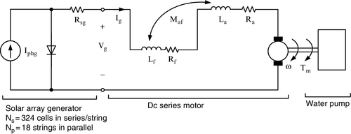
The solar array is governed by the relation

where Vg is the output voltage and Ig is the output current of the solar array. The current Iphg is the photon current, which is proportional to the insolation Q. The value Iphg = 13.6 A corresponds to 100% of insolation, that is, Q = 1000 W/m2.
The series DC motor has the rated parameters Vrat = 120 V, Irat = 9.2 A, nrat = 1500 rpm, Ra = 1.5 Ω, Rf = 0.7 Ω, Maf = 0.0675 H and can be described by the relation

where R = Ra + Rf and Tm = MafIa2.
The mechanical load (water pump) can be described by the relation
where A = 0.2 Nm, B = 0.0002387 Nm/(rad/s), and TL1 = 4.0 Nm.
a) Plot the solar array characteristic Ig versus Vg for the three insolation levels of Q = 100%, 80%, and 60% using Eq. P16-1 with Iphg as parameter.
b) Based on Eqs. P16-2 and P16-3 plot the motor torque relation (Eq. P16-2) and the water pump torque relation (Eq. P16-3) in the angular velocity (ω) versus torque (Tm) plane.
c) Using the relations Vm = Vg = MafIaω + RIa and Tm = MafIa2, where Ia = Ig, plot the load line Tm1 in the Ig–Vg plane. Does a good load matching exist?
d) Calculate the input power of the series DC motor Pin from Vrat and Irat.
e) Calculate the power delivered to the pump by the solar array Psolar at Q = 100%, 80%, and 60% insolation.
f) How does Ρsolar compare with Ρin for the three different insolation levels?
Problem 8.17: Design of a 5 MW Variable-Speed Wind-power Plant for an Altitude of 1600 m
Design a wind-power plant supplying the rated power Pout = 5 MW into the three-phase distribution system at a line-to-line voltage of VL–L system = 12.47 kV. The wind-power plant consists of the following:
• One (Y-grounded/Δ) three-phase, step-up transformer, Ninverter parallel-connected three-phase PWM inverters with an input voltage of VDC = 1200 V, where each inverter delivers an output AC current Iphase_inverter at unity power factor cosΦ = 1 to the low-voltage winding of the transformer (e.g., the angle Φ between the line-to-neutral voltage of the inverter VL-n_inverter and the phase current of the inverter Iphase_inverter is zero).
• Nrectifier (= Ninverter) three-phase rectifiers, each one equipped with one self-commutated switch and 6 diodes operating at a duty cycle of δ = 0.5. Note that each rectifier feeds one inverter.
• One synchronous generator.
• One mechanical gear.
• One wind turbine.
a) Sketch the block diagram of the entire windpower plant. At rated operation, the efficiencies of (one) gear box, (one) generator, (one) rectifier, (one) inverter, and (one) transformer are η = 0.95, each. Note there are Nrectifier parallel rectifiers and Ninverter parallel inverters. At an operation of less than rated load the efficiencies will be smaller. The parallel configuration of inverters and rectifiers permits an efficiency increase, because at light and medium loads only a few inverters and rectifiers must be operated, and some can be disconnected.
b) Determine the output power of each component, e.g., transformer, inverters, rectifiers, generator, gear box, wind turbine, at rated operation.
c) Determine for a modulation index of m = 0.8 the inverter output line-to-neutral voltage VL-n inverter such that the inverter can deliver at unity power factor an approximately sinusoidal current to the transformer. Ninverter commercially available three-phase PWM inverters are connected in parallel and one inverter has the output power rating Pinverter = 500 kW. What is the number of inverters required? Determine Iphase_inverter of one inverter, the resulting output current of all Ninverter inverters, that is, Σ Iphase_inverter, and the transformation ratio a = (Ns/Np) of the (Y-grounded/Δ) step-up transformer. For your calculations you may assume (one) ideal transformer and an ideal power system, where all resistances and leakage inductances are neglected. However, the resistances of the transformer are taken into account in the efficiency calculation of the transformer. Why do we use a Y-grounded/Δ transformer configuration?
d) Each of the Ninverter inverters is fed by one three-phase rectifier with one self-commuted PWM-operated switch (IGBT) and 6 diodes, and all Nrectifier three-phase rectifiers are fed by (one) three-phase synchronous generator with p = 8 poles at ns = 900 rpm, utilization factor C = 3.5 kWmin/m3, Drotor = 1.0 m. The input line-to-line voltage VL–L rectifier = 1.247 kV of one three-phase rectifier results at a duty cycle of δ = 0.5 in the DC output voltage (of one rectifier, including filter) VDC = 1200 V. Determine the line-to-line output voltage VL–L generator of the nonsalient-pole (round-rotor) synchronous generator such that it matches the required input line-to-line voltage of the rectifier VL–L rectifier; thus a transformer between synchronous generator and rectifier can be avoided. Find all pertinent parameters of the synchronous generator including its synchronous reactance XS in per unit and in ohms.
e) Design the mechanical gear between wind turbine and synchronous generator so that the wind turbine can operate at nturbine = 10 rpm.
f) Determine the geometric dimensions of the wind turbine – using the Lanchester–Betz-Joukowsky equation – for the power efficiency coefficient cp = 0.4 of the wind turbine, and the rated wind velocity of v = 8 m/s.
g) What are the advantages and disadvantages of this variable-speed wind-power plant design?