9.3.1 Filter Transfer Function

Transfer functions are extensively used for filter design and system modeling. Figure 9.4a shows the single-phase presentation of a balanced three-phase distribution system with a nonlinear load and a passive shunt filter installed at the PCC. At harmonic frequencies, the system can be approximated by the equivalent circuit of Fig. 9.4b. Three main types of transfer functions can be defined: impedance, current-divider, and voltage-divider transfer functions.

9.3.2 Common Types of Passive Filters for Power Quality Improvement

The configuration of a filter depends on the frequency spectrum and nature of the distortion. Figure 9.5 depicts common types of passive filters.

The first-order damped and undamped high-pass filter (Fig. 9.5a with and without the resistor, respectively) is used to attenuate high-frequency current harmonics that cause telephone interference, reduce voltage notching caused by commutation of SCRs or thyristors, and provide partial displacement power factor correction of the fundamental load current. The single-tuned low-pass (also called band-pass or second-order series resonant band-pass) filter (Fig. 9.5b) is most commonly applied for mitigation of a single dominant low-order harmonic. Fig. 9.5c represents a second-order damped high-pass filter. Most nonlinear loads and devices generate more than one harmonic, however, and one filter is not usually adequate to effectively compensate, mitigate, or reduce all harmonics within the power system. There are different approaches to overcome this problem.

One approach is to use two single-tuned filters with identical characteristics to form a double bandpass filter (Fig. 9.5d). In practice, there is more than one dominant low-order harmonic and combinations of three or more single-tuned filters are applied. Starting with the lowest harmonic order (e.g., 5th), each filter is tuned to one harmonic frequency. This approach is not practical when the number of dominant low-order harmonics is large and/or higher order harmonics are present.

Another approach is to use a first-order high-pass filter (consisting of a resistor connected in series with a capacitor) or a second-order high-pass filter (consisting of a series capacitor and a parallel combination of inductor and resistor; Fig. 9.5c) and set the resonant frequency below the lowest order dominant harmonic frequency. However, the (Z – ω) plot of a second-order high-pass filter shows that the minimum impedance of this filter (e.g., in the pass-band region) is higher than that of a single-tuned band-pass filter. Therefore, the high-pass filter allows a percentage of all harmonics above its notch frequency to pass through and will result in large fundamental filter rating and high resistive losses. This filter is commonly applied for higher frequencies and notch reduction.

The third and most implemented approach is to install a composite filter consisting of two or more branches of band-pass filters tuned at low-order harmonic frequencies and a parallel branch of high-pass filter tuned at higher frequencies (called a passive filter element; Figs. 9.5e, 9.11, and 9.12). This configuration is suitable for most residential, domestic, and industrial nonlinear loads such as arc furnaces. In addition, there are other configurations of higher order filters (e.g., third-order damped filter) for transmission systems.

The following section derives the equations and general relations of basic filter types.

9.3.2.1 First-Order, High-Pass Filter

A first-order, high-pass filter consists of a shunt capacitor (Fig. 9.6a) and can be used to attenuate high-frequency harmonic current components causing telephone interference, to reduce voltage notching (e.g., caused by rectifier commutation), and to improve the displacement (fundamental) load power factor. Such filters are amply described in currently available circuit textbooks [12,13].

If the system impedance is purely inductive (Z_sys(s) = sL_sys), filter impedance and filter system impedance transfer functions can be derived using Eqs. 9-1:

$H_f\left(s\right)=Z_f\left(s\right)=\frac{V_f\left(s\right)}{I_f\left(s\right)}=\frac{1}{s{C}_f}\text{,}$

  (9-4a)

$\begin{array}{c}{H}_{\mathit{fsys}}\left(s\right)=Z_{\mathit{fsys}}\left(s\right)=\frac{V_{sys}\left(s\right)}{I_f\left(s\right)+I_{sys}\left(s\right)}=\frac{1}{\frac{1}{Z_f\left(s\right)}+\frac{1}{Z_{sys}\left(s\right)}}=\frac{1}{s{C}_f+\frac{1}{s{L}_{sys}}}\text{.}\end{array}$

  (9-4b)

The order of this filter, that is, the highest exponent of the characteristic (denominator) polynomial of H_f (s), is one.

The current-divider transfer function, Eq. 9-2a, can be derived as

$H_{cds}\left(s\right)=H_{cds}\left(j\omega \right)=\frac{\frac{1}{j\omega C_f}}{j\omega L_{sys}+\frac{1}{j\omega C_f}}\text{.}$

  (9-5)

Simple algebra yields analytical (closed-form) expressions for asymptotes, local maxima, and minima of these transfer functions as is illustrated in Fig. 9.6b,c. The procedures for plotting H_cds(jω) on a logarithm paper as shown in Fig. 9.6c are

• For low frequencies $\left(\omega <<1/\sqrt{L_{sys}{C}_f}\Rightarrow |1/j\omega C_f|>>||j\omega L_{sys}|\right):$

$H_{cds}\left(j\omega \right)\approx \frac{\frac{1}{j\omega C_f}}{\frac{1}{j\omega C_f}}=1\text{.}$

Therefore, the roll-off of the low-frequency components is one or 0 dB per decade.

• For high frequencies $\left(\omega >>1/\sqrt{L_{sys}{C}_f}\Rightarrow |1/j\omega C_f|<<||j\omega L_{sys}|\right):$

$H_{cds}\left(j\omega \right)\approx \frac{\frac{1}{j\omega C_f}}{j\omega L_{sys}}=\frac{-1}{{\omega }^2{L}_{sys}{C}_f}\text{.}$

Therefore, the roll-off of the high frequency components is 1/ω² or −40 dB per decade.
If system resistance is included (Z_sys(s) = R_sys + sL_sys), the maximum can be found as

$H_{cds}\left(s=j\omega \right)|{}_{\omega =\frac{1}{\sqrt{L_{sys}{C}_f}}}=-j\frac{1}{R_{sys}}\sqrt{\frac{L_{sys}}{C_f}}$

and

$\begin{array}{l}{H}_{\mathit{max}}=|H_{cds}\left(s=j\omega \right)|{}_{\omega =\frac{1}{\sqrt{L_{sys}{C}_f}}}\\ \mathrm{with}\mathrm{the}\mathrm{quality}\mathrm{factor}\\ Q=\frac{1}{R_{sys}}\sqrt{\frac{L_{sys}}{C_f}},\mathrm{therefore},H_{\mathit{max}}=Q\text{.}\end{array}$

Similar procedures are relied on to plot H_fsys(jω) as shown in Fig. 9.6b.

9.3.2.2 First-Order Damped High-Pass Filter

Figure 9.7a shows the configuration of a first-order damped high-pass filter. A series connected resistance (R_f) is included to provide a damping characteristic.

Filter transfer functions are

$H_f\left(s\right)=Z_f\left(s\right)=\frac{V_f\left(s\right)}{I_f\left(s\right)}=R_f+\frac{1}{s{C}_f}\text{.}$

  (9.6a)

$H_{\mathit{fsys}}\left(s\right)=Z_{\mathit{fsys}}\left(s\right)=\frac{1}{\frac{1}{R_f+1/s{C}_f}+\frac{1}{s{L}_{sys}}}\text{,}$

  (9.6b)

$H_{cds}\left(s\right)=H_{cds}\left(j\omega \right)=\frac{R_f+\frac{1}{j\omega C_f}}{R_f+\frac{1}{j\omega C_f}+j\omega L_{sys}}\text{.}$

  (9.6c)

As discussed in the previous section, H_cds(s) can be determined analytically (Fig. 9.7c):

• For low frequencies $\left(\omega <<1/\sqrt{L_{sys}{C}_f}\Rightarrow |1/j\omega C_f|>>|j\omega L_{sys}|\right):$

$H_{cds}\left(j\omega \right)\approx \frac{\frac{1}{j\omega C_f}}{\frac{1}{j\omega C_f}}=1\text{.}$

• For moderate high frequencies $\left(1/\sqrt{L_{sys}{C}_f}<\omega <1/R_f{C}_f\Rightarrow |1/j\omega C_f|<<|j\omega L_{sys}|\right):$

$\begin{array}{c}{H}_{cds}\left(j\omega \right)\approx \frac{\frac{1}{j\omega C_f}}{j\omega L_{sys}}=\frac{-1}{{\omega }^2{L}_{sys}{C}_f}\\ \Rightarrow \mathrm{roll}-\mathrm{off}\mathrm{is}1/{\omega }^2\mathrm{or}–40\mathrm{dB}\mathrm{per}\mathrm{decade}\text{.}\end{array}$

• For high frequencies (ω > > 1/R_fC_f ⇒ R_f > > |1/jωC_f| and |jωL_sys| > > |R_f + 1/jωC_f|):

$\begin{array}{c}{H}_{cds}\left(j\omega \right)=\frac{R_f+\frac{1}{j\omega C_f}}{j\omega L_{sys}+\left(R_f+\frac{1}{j\omega C_f}\right)}\approx \frac{R_f}{j\omega L_{sys}}\\ \Rightarrow \mathrm{roll}-\mathrm{off}\mathrm{is}1/\omega \mathrm{or}–20\mathrm{dB}\mathrm{per}\mathrm{decade}\text{.}\end{array}$

• If the system resistance is included (Z_sys(s) = R_sys + sL_sys), the maximum can be found as

$H_{cds}\left(s=j\omega \right)|{}_{\omega =\frac{1}{\sqrt{L_{sys}{C}_f}}}=1-j\frac{1}{R_{sys}}\sqrt{\frac{L_{sys}}{C_f}}$

and

$H_{\mathit{max}}=|H_{cds}\left(s=j\omega \right)|{}_{\omega =\frac{1}{\sqrt{L_{sys}{C}_f}}}=\sqrt{Q^2+1}\approx Q$

with the quality factor $Q=\frac{1}{R_{sys}}\sqrt{\frac{L_{sys}}{C_f}}\text{.}$

Similar procedures are employed to plot H_fsys(jω) as illustrated in Fig. 9.7b. Comparison of Figs. 9.6 and 9.7 indicates the following:

• the damping resistance significantly limits the high-frequency performance (e.g., roll-off of high-frequency components is only 1/ω or −20 dB per decade). Therefore, the damped filter is less desirable for telephone interference reduction applications; and

• for parallel resonant conditions (e.g., cancellation of L_sys by C_f), if the resonant frequency falls on or near a critical harmonic frequency, a high-pass damping resistance (R_f) can be used to control and reduce the amplification. However, this will increase the fundamental frequency power loss and reduces the effectiveness of the high-pass attenuation above the frequency 1/(R_fC_f).

9.3.2.3 Second-Order Band-Pass Filter

The second-order band-pass filter (also called single-tuned or series-resonant filter) is a series combination of capacitor (C_f), inductor (L_f), and a small damping resistor (R_f), as depicted in Fig. 9.8a. The damping resistance is usually due to the internal resistance of either the inductor and/or capacitor. This filter is tuned to attenuate one single low-order harmonic. Typically, combinations of band-pass filters are used because the power system contains a number of dominant low-order harmonics.

Assuming a pure inductive system (Z_sys(s) = sL_sys), filter transfer functions can be derived using Eqs. 9-1a and 9-2a:

$\begin{array}{c}{H}_f\left(s\right)=Z_f\left(s\right)=\frac{V_f\left(s\right)}{I_f\left(s\right)}=R_f+s{L}_f+\frac{1}{s{C}_f}\\ =\frac{A}{s}\left[1+\frac{1}{Q}\left(\frac{s}{{\omega }_0}\right)+{\left(\frac{s}{{\omega }_0}\right)}^2\right]\text{,}\end{array}$

  (9-7)

$H_{cds}\left(s\right)=H_{cds}\left(j\omega \right)=\frac{R_f+j\omega L_f+\frac{1}{j\omega C_f}}{R_f+j\omega L_f+\frac{1}{J\omega C_f}+j\omega L_{sys}}\text{.}$

  (9-8)

where A is the gain. The filter quality factor (Q) and the series-resonant frequency (ω₀) are

$Q=\frac{1}{R_f}\sqrt{\frac{L_f}{C_f}}\text{,}$

  (9-9a)

${\omega }_0=\frac{1}{\sqrt{L_f{C}_f}}\text{.}$

  (9-9b)

For high-voltage applications, the filter current has a low rms magnitude and does not require large current carrying conductors; therefore, air-core inductors are regularly used and the filter quality factor is relatively large (e.g., 50 < Q < 150). For low-voltage applications, gapped iron-core inductors and conductors with a large cross section are employed (e.g., 10 < Q < 50).

The filter impedance transfer function H_f (jω) is presented graphically as shown in Fig. 9.8b. It is evaluated at low and high frequencies to determine its asymptotes:

• At low frequencies (ω << ω₀ ⇒ |1/jωC_f |>> |R_sys + jωL_sys|), the filter is dominantly capacitive and provides reactive power to the system. Therefore, H_f(s) ≈ 1/jωC_f and the roll-off of the low frequency components is −20 dB per decade.

• At high frequencies (ω >> ω₀ ⇒ |jωL_sys| >> |R_f + 1/jωC_f|), the filter is dominantly inductive and consumes reactive power with little influence on high-frequency distortions. Therefore, H_f(s) ≈ jωL_f and the roll-off of the high frequency components is + 20 dB per decade.

• At the resonant frequency (ω = ω₀), the filter is entirely resistive, that is, H_f(s) = R_f. More attenuation is provided with lower filter resistances; however, there are practical limits to the value of R_f.

Similar procedures are applied to plot H_fsys(jω) and H_cds(jω) as illustrated in Fig. 9.8c,d, respectively. Note that the minima of the transfer functions (H_min) are very close to the series resonant frequency; however, due to the interaction between the capacitive reactance and the filter inductive reactance, H_max does not occur at the parallel resonant frequency formed by filter capacitance and system inductance. The derivatives of the transfer functions are usually evaluated numerically to determine frequencies where maxima occur.

The second-order band-pass (series resonant) filters are very popular and have many applications in power system design including transmission (e.g., connected in parallel at the AC terminals of HVDC converters), distribution (e.g., for detuning power factor capacitor banks to avoid parallel resonant frequencies), and utilization (e.g., across terminals of nonlinear loads).

9.3.2.4 Second-Order Damped Band-Pass Filter

A popular topology of the second-order damped filter is shown in Fig. 9.9a where a bypass resistance (R_bp) is included across the inductor to provide attenuation for harmonic frequency components over a wide frequency range. The filter impedance transfer function can be expressed in normalized form

$\begin{array}{c}{H}_f\left(s\right)=Z_f\left(s\right)=\frac{V_f\left(s\right)}{I_f\left(s\right)}=\frac{1}{\frac{1}{R_{\mathit{bp}}}+\frac{1}{R_f+s{L}_f}}+\frac{1}{s{C}_f}\\ =\frac{A}{s\left(1+\frac{s}{{\omega }_p}\right)}\left[1+\frac{1}{Q_{\mathit{bp}}}\left(\frac{s}{{\omega }_0}\right)+{\left(\frac{s}{{\omega }_0}\right)}^2\right]\text{,}\end{array}$

  (9-10a)

where the gain A, the series resonant angular frequency ω₀, the quality factor Q_bp, and the pole frequency ω_p [13] for typical cases (whereby R_f << R_bp) are

$\begin{array}{l}A=\frac{1}{C_f},{\omega }_0=\sqrt{\frac{R_f+R_{\mathit{bp}}}{R_{\mathit{bp}}{L}_f{C}_f}}\approx \frac{1}{\sqrt{L_f{C}_f}},\\ Q_{\mathit{bp}}=\frac{R_f+R_{\mathit{bp}}}{{\omega }_0\left(R_{\mathit{bp}}{R}_f{C}_f+L_f\right)},{\omega }_p=\frac{R_f+R_{\mathit{bp}}}{L_f}\approx \frac{R_{\mathit{bp}}}{L_f}\text{.}\end{array}$

  (9-10b)

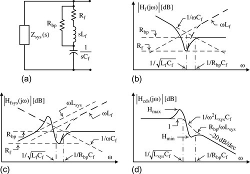
The series resistance R_f is determined by the desired quality factor of the second-order band-pass filter, and R_bp is selected to achieve the required high-pass response and series resonant attenuation. Typical values of the bypass quality factor are 0.5 < Q_bp < 2.0. However, there is a trade-off between larger values (e.g., more series resonant attenuation and less high-pass response) and smaller values (e.g., less series resonant attenuation and greater high-pass response) of the quality factor.

9.3.2.5 Composite Filter

Higher order filters are constructed by increasing the number of storage elements (e.g., capacitors, inductors). However, their application in power systems is limited due to economic and reliability factors.

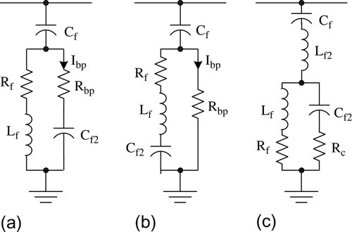
A third-order filter may be constructed by adding a series capacitance C_f2 to the inductor bypass resistance (Fig. 9.10a) to limit I_bp and reduce the corresponding fundamental frequency losses or by including C_f2 in series with L_f (Fig. 9.10b) and sizing it to form a series resonant branch at the fundamental frequency to reduce I_bp and to increase filter efficiency. If a second inductor L_f2 is added to the circuit of Fig. 9.10a, a fourth-order double band-pass filter will be obtained, as shown in Fig. 9.10c.

A common type of an nth-order composite filter for power quality improvement is shown in Fig. 9.11. Several band-pass filters are connected in parallel and individually tuned to selected harmonic frequencies to provide compensation over a wide frequency range. The last branch is a high-pass filter attenuating high-order harmonics, which usually are a result of fast switching actions. Composite filters are only applied when even-order harmonics are small since a parallel resonance will occur between any two adjacent band-pass filter branches and cause amplification of the distortion in that frequency range. For example, composite filter systems with shunt branches tuned at the 5th and 7th harmonics will have a resonant frequency at about the 6th harmonic. The impedance transfer function of the nth-order composite filter is

$\begin{array}{c}{H}_f\left(s\right)=Z_f\left(s\right)=\frac{V_f\left(s\right)}{I_f\left(s\right)}=\frac{1}{\frac{1}{Z_f^{\left(5\right)}}+\frac{1}{Z_f^{\left(7\right)}}+\frac{1}{Z_f^{\left(11\right)}}+....+\frac{1}{Z_f^{\left(n\right)}}}\text{.}\end{array}$

  (9-11)

It is time-consuming to derive the transfer functions of multiple-order filters in terms of factorized expressions of poles and zeros [13]. Therefore, numerical approaches are typically applied to plot the transfer function, and an iterative design procedure is used to optimize a filter configuration.

9.3.3 Classification of Passive Power Filters

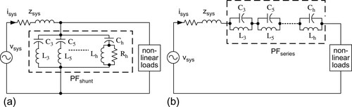
Passive filters cause harmonic currents to flow at their resonant frequency. Due to this resonance, the harmonic currents are attenuated in the power system through the LC filter circuits tuned to the harmonic orders that require filtering. In practice, a single passive filter is not adequate since there is more than one harmonic to be attenuated; therefore, a shunt or series passive composite filter unit (Fig. 9.12) is used. Passive filter units are generally designed to remove a few low-order harmonics, for example, the 5th, 7th, and 11th. Normally passive filter units employ three (or more for high-power applications such as HVDC) tuned filters, the first two being for the lowest dominant harmonics followed by a high-pass filter. In a shunt passive filter unit, two lossless LC components are connected in series to sink harmonic currents and all three (or more) filters are connected in parallel (Fig. 9.12a). However, in a series passive filter unit, two lossless LC components are connected in parallel for creating a harmonic dam and all three (or more) filters are connected in series, as shown in Fig. 9.12b.

The inductors should have high quality factors to reduce system losses and must not saturate in the entire current operating region. Capacitor values are decided by the required reactive power of the system, and then inductor values are calculated by tuning them for the particular harmonic frequencies. Resistor values are calculated by the corresponding quality factors based on the desired sharpness of the characteristics. Similarly, the resistance of the high-pass filter is computed based on the sharpness or attenuation of the higher order harmonics on the one hand, and reducing the losses on the other hand to achieve an optimum value for the quality factor. Passive filter units with shunt and series configurations are extensively used in single-phase (Fig. 9.13), three-phase three-wire (Fig. 9.14), and three-phase four-wire (Fig. 9.15) systems to improve the quality of power and mitigate harmonic currents and voltages.

9.3.4 Potentials and Limitations of Passive Power Filters

Design, construction, and implementation of passive filters are straightforward and easier than their counterparts, for example, synchronous condensers and active filters. They have many advantages:

• they are robust, economical, and relatively inexpensive;

• they can be implemented in large sizes of MVArs and require low maintenance;

• they can provide a fast response time (e.g., one cycle or less with static voltage converter, SVC), which is essential for some power quality problems such as flickering voltage dips due to arc-furnace loads;

• unlike rotating machines (e.g., synchronous motors or condensers) passive filters do not contribute to the short-circuit currents; and

• in addition to power quality improvement, well-designed passive filters can be configured to provide power factor correction, reactive power compensation, or voltage support (e.g., on critical buses in case of a source outage) and reduce the starting impact and associated voltage drops due to large loads (e.g., large induction motors).

These advantages have resulted in broad applications of passive filters in different sectors of power systems. However, power engineers have also encountered some limitations and shortcomings of passive filters, which have called for alternative solutions such as active and hybrid filter systems. Some limitations of passive filters are as follows:

• fixed compensation or harmonic mitigation, large size, and possible resonance with the supply system impedance at fundamental and/or other harmonic frequencies;

• compensation is limited to a few orders of harmonics;

• once installed, the tuned frequency and/or filter size cannot be changed easily;

• unsatisfactory performance (e.g., detuning) may occur due to variations of filter parameters (caused by aging, deterioration, and temperature effects) and nonlinear load characteristics;

• change in system operating conditions (e.g., inclusion of capacitors and/or other filters) has large influence on filter designs. Therefore, to be effective, filter impedance should be less than system impedance, which can become a problem for strong or stiff systems [2];

• resonance between system and filter (e.g., shifted resonance frequency) for single- and double-tuned filters can cause an amplification of characteristics and noncharacteristic harmonic currents. Therefore, the designer has a limited choice in selecting tuned frequencies and ensuring adequate bandwidth between shifted frequencies and integer (even and odd) harmonics [2];

• special protective and monitoring devices might be required to control switching surges, although filter reactors will reduce the magnitude of the switching inrush current magnitude and its associated high frequency; and

• stepless control (of reactive power, power factor correction, and voltage support) is not possible since the filter can either be switched on or switched off only.

9.3.5 Application Example 9.1: Hybrid Passive Filter Design to Improve the Power Quality of the IEEE 30-Bus Distribution System Feeding Adjustable-Speed Drives

Consider the IEEE 23 kV, 30-bus distribution system [9,10] shown in Fig. E9.1.1. System transmission-line data, bus data, and capacitor data are provided in Tables E9.1.1 to E9.1.3, respectively. To investigate the impact of large AC drive systems on the power quality of the distribution system, a PWM adjustable-speed drive (675 kW, 439 kVAr) and a variable-frequency drive (350 kW, 175 kVAr) are connected to buses 15 and 18, respectively. Table E9.1.4 depicts the spectra of the current harmonics injected by typical AC drives into the system. Use harmonic current sources to model the two nonlinear loads and utilize the decoupled harmonic power flow algorithm (Chapter 7, Section 7.5.1) to simulate the system. Determine the total harmonic voltage distortion (THD_v) of the system and at the individual buses before and after the installation of the hybrid passive filter banks listed below. Plot the voltage and current waveforms at bus 15 before and after filtering.

a) Two filter banks are placed at the terminals of nonlinear loads (buses 15 and 18). Each bank consists of a number of shunt-connected series resonance passive filters tuned at the respective dominant harmonic frequencies. Assume R_f = 100 Ω and L_f = 100 mH for all filters and compute the corresponding values of C_f.

b) Repeat part a with one filter bank at bus 15.

c) Repeat part b with one filter bank at bus 9.

d) Compare the results of parts a to c and make comments regarding the impact of numbers and locations of filters on the power quality of the system.

Solution to Application Example 9.1

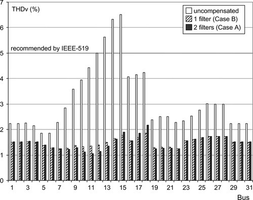
a) Case A. Harmonic Compensation with Two Hybrid Passive Filter Banks at Buses 15 and 18. Harmonic analysis before the installation of passive filters indicates a very high distortion of both voltage and current waveforms (Fig. E9.1.3 and Table E9.1.5) due to the two AC drives with relatively high power ratings. According to the IEEE-519 standard [11], the individual harmonic current injections at bus 15 (for 5th, 7th, 11th, 13th, 17th, and 19th harmonics) and bus 18 (for 5th, 7th, and 11th harmonics) are higher than the allowable level of 4%, and thus the electric utility has the right to disconnect (reject) these nonlinear loads. In addition, propagation of the injected harmonic currents has resulted in unacceptable voltage THD_v levels (e.g., larger than 5%) at buses 12 to 15. Buses 11 and 16 to 18 are also experiencing relatively high THD_v of more than 4% (see Fig. E9.1.6).
The common procedure is to require the owners of nonlinear loads (at buses 15 and 18) to install passive filter banks at the terminals of the AC drives. Figure E9.1.3 and Table E9.1.5 list the simulation results after the installation of the following two filter banks (Fig. E9.1.2), tuned at the dominant frequencies:

• Filter Bank 1: Passive filter (Fig. E9.1.2) consisting of five shunt branches tuned to the 5th, 7th, 11th, 13th, and 17th harmonic frequencies and installed at bus 15 with (Eq. 9-9b with f₁ = 50 Hz)

$\begin{array}{c}{R}_f=100\mathrm{\Omega },L_f^{\left(h\right)}=100\mathrm{mH}\left(\mathrm{f}\mathrm{o}\mathrm{r}\mathrm{all}\mathrm{branches}\right),\\ {\omega }_n^{\left(\mathrm{h}\right)}=2\pi hf=1/\sqrt{L_f^{\left(h\right)}{C}_f^{\left(h\right)}}\Rightarrow C_f^{\left(5\right)}\Rightarrow 4.053\mu \mathrm{F},\\ {\mathrm{C}}_{\mathrm{f}}^{\left(7\right)}=2.068\mu \mathrm{F},C_f^{\left(11\right)}=0.837\mu \mathrm{F},{\mathrm{C}}_f^{\left(13\right)}=0.680\mu \mathrm{F},C_f^{\left(17\right)}=0.351\mu \mathrm{F}\text{.}\end{array}$

• Filter Bank 2: Passive filters (Fig. E9.1.2) with only two shunt branches tuned to the 5th and 7th harmonic frequencies and installed at bus 18 with (Eq. 9-9b with f₁ = 50 Hz)

$\begin{array}{c}{R}_f=100\mathrm{\Omega },L_f^{\left(h\right)}=100\mathrm{mH}\left(\mathrm{f}\mathrm{o}\mathrm{r}\mathrm{all}\mathrm{branches}\right),\\ {\omega }_n^{\left(h\right)}=2\pi hf=1/\sqrt{L_f^{\left(h\right)}{C}_f^{\left(h\right)}}\Rightarrow C_f^{\left(5\right)}\Rightarrow 4.053\mu \mathrm{F},{\mathrm{C}}_f^{\left(7\right)}=2.068\mu \mathrm{F}\text{.}\end{array}$

According to Table E9.1.5 the performance of the above filters is satisfactory: the maximum level of THD_v has dropped from 6.51 (at bus 15) to 2.17% (at bus 18) while the average system THD_v is within the permissible limits of the IEEE-519 standard [11].

b) Case B. Harmonic Compensation with One Passive Filter Bank at Bus 15. This case examines the possibility of meeting IEEE-519 [11] limits with only one filter bank. Simulation results before and after the installation of Filter Bank 1 at bus 15 are shown in Fig. E9.1.4 and Table E9.1.5. Therefore, by performing harmonic load flow analysis, it may be possible to eliminate unnecessary filter banks, and therefore reduce the overall cost of harmonic compensation.

c) Case C. Harmonic Compensation with One Passive Filter Bank at Bus 9. To show the impact of filter location on the overall power quality of the distribution system, Filter Bank 1 is installed between the two drive systems at bus 9. The resulting voltage and current waveforms are depicted in Fig. E9.1.5 and the corresponding THD_v levels are listed in Table E9.1.5. It is clear that improper placement of filters will not only deteriorate their performances, but might also favor harmonic propagation and cause additional power quality problems in other sectors of the system (e.g., in buses 10 to15 and 16 to 18 for Case C).

d) Comparison of Results. A comparison of the THD_v levels as well as the rms voltage values before and after the placement of filters (Cases A, B, and C) is listed in Table E9.1.5 and shown in Fig. 9.1.6.

The decoupled harmonic power flow algorithm (Chapter 7, Section 7.5.1) is used to simulate the distribution system. Nonlinear AC drives are modeled with harmonic current sources. This approach is very practical and convenient for the analysis of large distorted industrial systems with inadequate information about the nonlinear loads (e.g., parameters and ratings of AC drives). Simulation results of this application example indicate that the common approach of placing filter banks at the terminals of each AC drive system is not always the most economical solution. It might be possible to limit the overall system distortion, as well as the individual bus THD_v levels, with fewer filters. To do this, system conditions before and after compensation need to be carefully studied, which requires fast algorithms, as presented in this example.

9.4.1 Classification of Active Power Filters Based on Topology and Supply System

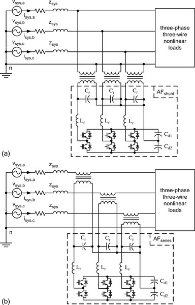
Active filters have become a mature technology for harmonic and reactive power compensation of single- and three-phase electric AC power networks with high penetration of nonlinear loads. This section classifies active filters based on the supply system taking into consideration their (shunt or/and series) topology. Therefore, there are six types of shunt and series connected active filters for single-phase two-wire, three-phase three-wire, and three-phase four-wire AC networks, as shown in Figs. 9.16, 9.17, and 9.18, respectively. Composite filters consisting of two or more active filters are realized as hybrid filters and are discussed in Section 9.5.

9.4.2 Classification of Active Power Filters Based on Power Rating

Active filters can also be classified according to their power rating and speed of response required for their application in a compensated system [5]:

• Low-power active filters (with power ratings below 100 kVA and response times of about 10 μs to 10 ms) are mainly used in residential areas, small to medium-sized factories, electric drives, commercial buildings, and hospitals. These applications require sophisticated dynamic filtering techniques and include single-phase and three-phase systems.

• Single-phase active filters are mainly available for low power ratings, and hence can be operated at relatively high frequencies leading to improved performance and lower prices. They have many retrofit applications such as commercial and educational buildings with many computer loads.

• For balanced three-phase low power applications a three-phase filter can be used. However, for unbalanced load currents or unsymmetrical supply voltages, especially in three-phase four-wire distribution systems, three single-phase filters or a hybrid filter are usually required.

• Medium-power active filters (with power ratings of about 100 kVA to 10 MVA and response times of about 100 ms to 1 s) are mainly associated with medium- to high-voltage distribution systems and high-power, high-voltage drive systems, where the effect of phase imbalance is negligible. Due to economic concerns and problems associated with high-voltage systems (isolation, series or parallel connections of switches, etc.), these filters are usually designed to perform harmonic cancellation, and reactive-power compensation is not included in their control algorithms. At high voltage, other approaches of reactive power compensation such as capacitive or inductive static compensators, synchronous condensers, controlled LC filters, tuneable harmonic filters, line-commutated thyristor converters, and VAr compensators should be considered.

• High-power active filters (with power ratings above 10 MVA and response times of tens of seconds) are mainly associated with power-transmission grids, ultrahigh-power DC drives, and HVDC. Due to the availability of high switching-frequency power devices with high-voltage and high-power ratings, these filters are not cost effective. It is possible to use series–parallel combinations of low-power switches; however, there are many implementation issues and cost considerations. Fortunately, there are not too many power quality problems associated with high-voltage power systems.

9.5.1 Classification of Hybrid Filters

Hybrid filters combine a number of passive and/or active filters and their structure may be of series or parallel topology or a combination of the two. They can be installed in single-phase, three-phase three-wire, and three-phase four-wire distorted systems. The passive circuit performs basic filtering action at the dominant harmonic frequencies (e.g., 5th or 7th) whereas the active elements, through precise control, mitigate higher harmonics. This will effectively reduce the overall size and cost of active filtering.

In the literature, there are different classifications of active and hybrid filters based on power rating, supply system (e.g., number of wires and phases), topology (e.g., shunt and/or series connection), number of (passive and active) elements, speed of response, power circuit configuration, system parameter(s) to be compensated, control approach, and reference-signal estimation technique. In this book, classification of hybrid filters is based on the supply system with the topology as a further subclassification. If there are a maximum of three (passive and active) filters in each phase, then 156 types of hybrid filters are expected for single-phase two-wire systems, three-phase three-wire, and three-phase four-wire AC networks. Figures 9.19 to 9.25 show the 52 types of hybrid filter topologies for single-phase two-wire systems. These topologies can be easily extended to illustate the other 104 types of hybrid filters for three-phase systems.

Figures 9.19 and 9.20 depict hybrid filters consisting of two and three passive filters, respectively, whereas Figs. 9.21 and 9.22 show similar configurations for two and three active filters. There are 8 topologies of hybrid filters consisting of one passive and one active filter as shown in Fig. 9.23. There are many possible combinations if three filters are combined. Figure 9.24 illustrates the 18 possible hybrid filters consisting of two passive filters and one active filter. There are also 18 possible hybrid filters consisting of one passive filter and two active filters as represented in Fig. 9.25.

The rating of active filters is reduced through augmenting them by passive filters to form hybrid filters. This reduces the overall cost and in many cases provides better compensation than when either passive or active filters alone are employed. However, a more efficient approach is to combine shunt and series active filters, which can provide both current and voltage compensation. This (active–active) hybrid filter is known as a unified power quality conditioner (UPQC) or universal active filter (Fig. 9.21). Therefore, the development in hybrid filter technology began from the arrangement of (two or three) passive filters (Figs. 9.19 and 9.20) and progressed to the more effective combination of a number of shunt and/or series active filters (Figs. 9.21 to 9.25), yielding a cost-effective solution and complete compensation.

Hybrid filters are usually considered a cost-effective option for power quality improvement, compensation of the poor power quality effects due to nonlinear loads, or to provide a sinusoidal AC supply to sensitive loads. There are a large number of low-power nonlinear loads in a single-phase power system, such as ovens, air conditioners, fluorescent and LED lamps, TVs, computers, power supplies, printers, copiers, and battery chargers. Low-cost harmonic compensation of these residential nonlinear loads can be achieved using passive filters (Figs. 9.19 and 9.20). Compensation of single-phase high-power traction systems are effectively performed with hybrid filters (Figs. 9.21 and 9.22). Three-phase three-wire power systems are supplying a large number of nonlinear loads with moderate power levels – such as adjustable-speed drives – up to large power levels associated with HVDC transmission systems. These loads can be compensated using either a group of passive filters (e.g., a passive filter unit as shown in Fig. 9.13a) or a combination of active and passive filters of different configurations (Figs. 9.23 to 9.25) depending on the properties of the AC system.

9.7.1 Derivation of Reference Signal using Waveform Compensation

The objective of waveform compensation is to achieve a sinusoidal supply current. There are many signal-processing techniques that can be used to decompose the distorted waveform into its fundamental (to be retained) and harmonic (to be cancelled) components. This is essentially a filtering task; however, in addition to analytical approaches, there are also pattern-learning techniques that can be implemented.

9.7.1.1 Waveform Compensation using Time-Domain Filtering

Distortion identification is a filtering task that can be performed by time-domain techniques or by Fourier-based frequency decomposition. The nonideal properties of real filters such as attenuation (e.g., preserving the identified components and heavily attenuating other components with a narrow bandwidth), phase distortion (e.g., preserving the phase of the identified components), and time response (e.g., considering the time-varying nature of the distortion signal and enforcing rapid filter response without large overshoot) must be recognized. The performance considerations of time-domain filters are linked, for example, smoothness of the magnitude response has to be traded off versus the phase response, and a well-damped transient response is in conflict with a narrow transition region. There are two general approaches to identify the distortion components in the time domain (Fig. 9.27a):

• Direct distortion identification applies a high-pass filter to the distorted signal d(t) to determine the reference r(t). Therefore, the identification process is subject to the transient response of the filter.

• Indirect distortion identification uses the filter to determine the fundamental component f(t) and subtracts it from the distorted signal d(t) to form the reference r(t).

Due to the inherent time lag of actual filters, the distortion term of the direct method will be out of date and the distortion cancellation will be in error. The disadvantage of the indirect method is the out-of-date fundamental term that requires additional exchange of real power through the inverter, resulting in DC-bus voltage disturbance and increased rating of the inverter. Most active filters use indirect distortion identification to achieve the best distortion cancellation during transients. Direct methods are preferred in applications where specific ranges of harmonics are to be compensated or where different groups of harmonics are to be treated differently.

To facilitate the separation of fundamental and harmonic components of the signal, active filter control algorithms rely on transformation techniques to transfer the signal from the conventional three-phase abc reference frame to an orthogonal two-phase representation. This will reduce the burden of intensive computations. Two well-known transformations, the stationary αβ0 reference and the rotating dq0 reference (also called Park transformation) frames, are widely employed (see Fig. 9.27). The spectra of a nonlinear load current (supplied by undistorted sinusoidal supply voltage) in abc, αβ0, and dq0 reference frames are shown in Fig. 9.28a,b,c, respectively. Analysis of these graphs indicates:

• The nonlinear load is assumed to be three-wire, three-phase and unbalanced that injects harmonics of the order (6k ± 1), where k is any positive integer. This is clearly demonstrated by the frequency spectrum in the abc phase domain (Fig. 9.28a). Note that there is no distinction between harmonic components of the same order with different phase rotation.

• Both αβ0 and dq0 decompositions (Fig. 9.28b, c, respectively) transfer the zero-sequence component into a separate component set. Harmonic components with the same order and opposite phase rotation (e.g., –h and h) are separated because positive and negative sets are shifted to orders (h − 1) and –(h – 1), respectively.

• The αβ0 transformation (Fig. 9.28b) has no effect on the frequency spectra and does not separate sequence sets. The sequence can be determined from whether either the “α ” or the “β ” component leads. The negative harmonic term of order −1 indicates the imbalance of the fundamental. Balanced nonlinear loads produce characteristic harmonics of order −5, + 7, −11, + 13,…, 6k + 1. Unbalanced nonlinear loads generate in addition noncharacteristic harmonic components of order + 5, −7, + 11, −13, …, 6k −1.

• With the rotating dq0 transformation (Fig. 9.28c) all frequency components are shifted downward by one harmonic order. The positive-sequence fundamental becomes a DC term and the negative-sequence fundamental becomes a double-frequency term (order −2). The characteristic and noncharacteristic distortions are of orders 6k and (6k − 2), respectively.

• There is no difference between filtering in the abc or αβ0 domains, but the dq0 domain is a better alternative because it offers frequency separation of fundamental, positive, and negative sequences, which makes the filtering task simpler. In the abc domain the fundamental may be separated using a low-pass filter that cuts off between orders 1 and 5 (or 1 and 3 if there is zero-sequence/four-wire harmonic distortion). In the dq0 domain, the filter cutoff should be between 0 and 6 for balanced conditions. For unbalanced conditions, a cutoff between 0 and 2 will allow the negative-sequence (unbalanced) fundamental to be corrected and a cutoff between 2 and 4 will not cancel the unbalanced fundamental but will cancel harmonic distortion. Zero-sequence distortion is conveniently placed in a separate component set that may be cancelled or retained as required.

9.7.2 Derivation of Compensated Signals Using Instantaneous Power Compensation

Another approach to control active filters is to cancel the fluctuating component of instantaneous power and perhaps compensate the fundamental component of the reactive power. A common approach is to start with the definitions of instantaneous active and reactive powers and express them in terms of average and alternating (fluctuating) components. This can be performed in either the abc, αβ0, or dq0 domain:

• In the αβ0 domain:

$\left[\begin{array}{c}\hfill v_0\hfill \\ \hfill v_{\alpha }\hfill \\ \hfill v_{\beta }\hfill \end{array}\right]=\sqrt{\frac{2}{3}}\left[\begin{array}{ccc}\hfill 1/\sqrt{2}\hfill & \hfill 1/\sqrt{2}\hfill & \hfill 1/\sqrt{2}\hfill \\ \hfill 1\hfill & \hfill -1/2\hfill & \hfill -1/2\hfill \\ \hfill 0\hfill & \hfill \sqrt{3/2}\hfill & \hfill -\sqrt{3/2}\hfill \end{array}\right]\left[\begin{array}{c}\hfill v_a\hfill \\ \hfill v_b\hfill \\ \hfill v_c\hfill \end{array}\right]\text{.}$

Without the zero-sequence component, the instantaneous power can be written as

$\begin{array}{c}s\left(t\right)=p\left(t\right)+jq\left(t\right)=v_{\alpha \beta }{i}_{\alpha \beta }^{*}=\left(v_{\alpha }+j{v}_{\beta }\right)\left(i_{\alpha }-j{i}_{\beta }\right)\\ =\left(v_{\alpha }{i}_{\alpha }+v_{\beta }{i}_{\beta }\right)+j\left(v_{\beta }{i}_{\alpha }-v_{\alpha }{i}_{\beta }\right)\text{,}\end{array}$

where the superscript * denotes the complex conjugate. Therefore,

$\left[\begin{array}{c}\hfill p\hfill \\ \hfill q\hfill \end{array}\right]=\left[\begin{array}{c}\hfill \left(v_{\alpha }{i}_{\alpha }+v_{\beta }{i}_{\beta }\right)\hfill \\ \hfill \left(v_{\beta }{i}_{\alpha }-v_{\alpha }{i}_{\beta }\right)\hfill \end{array}\right]=\left[\begin{array}{cc}\hfill v_{\alpha }\hfill & \hfill v_{\beta }\hfill \\ \hfill v_{\beta }\hfill & \hfill -v_{\alpha }\hfill \end{array}\right]\left[\begin{array}{c}\hfill i_{\alpha }\hfill \\ \hfill i_{\beta }\hfill \end{array}\right]\text{.}$

• In the dq0 domain:

$\left[\begin{array}{c}\hfill v_d\hfill \\ \hfill v_q\hfill \\ \hfill v_0\hfill \end{array}\right]=\sqrt{\frac{2}{3}}\left[\begin{array}{ccc}\hfill \cos {\theta }_d\hfill & \hfill \cos \left({\theta }_d-2\pi /3\right)\hfill & \hfill \cos \left({\theta }_d+2\pi /3\right)\hfill \\ \hfill -\sin {\theta }_d\hfill & \hfill -\sin \left({\theta }_d-2\pi /3\right)\hfill & \hfill -\sin \left({\theta }_d+2\pi /3\right)\hfill \\ \hfill 1/\sqrt{2}\hfill & \hfill 1/\sqrt{2}\hfill & \hfill 1/\sqrt{2}\hfill \end{array}\right]\left[\begin{array}{c}\hfill v_a\hfill \\ \hfill v_b\hfill \\ \hfill v_c\hfill \end{array}\right]\text{.}$

In this equation θ_d = ω_d + φ, where ω_d is the angular velocity of voltages and φ is the initial voltage angle. With no zero-sequence components:

$\begin{array}{c}s\left(t\right)=p\left(t\right)+jq\left(t\right)\\ =v_{dq}{i}_{dq}^{*}=\left(v_d+j{v}_q\right)\left(i_d-j{i}_q\right)=\left(v_d{i}_d+v_q{i}_q\right)+j\left(v_q{i}_d-v_d{i}_q\right)\text{.}\end{array}$

In four-wire systems there is the additional term of zero-sequence instantaneous (real or reactive [6]) power; with Eqs. 9-13 and 9-15 the instantaneous power may be written as

$\begin{array}{c}p\left(t\right)=\overline{p}+\tilde{p}\left(t\right)\\ q\left(t\right)=\overline{q}+\tilde{q}\left(t\right)\text{.}\end{array}$

Figure 9.28a,d,e shows the spectra of current, active, and reactive powers for the case of a sinusoidal supply voltage, which is harmonically distorted and generates unbalanced currents. Characteristic harmonics of order h = 6k + 1 (e.g., −11, −5, 7, 13, …, where negative orders represent negative-sequence harmonics) produce power terms of order 6|k|, whereas noncharacteristic harmonics of order h = 6k − 1 (e.g., −13, −7, 5, 11,…) yield power terms of order 6|k| ± 2.

The inverse transform (e.g., conversion from power domain to the phase domain) is

$i_{\alpha \beta }^{*}=i_{\alpha }-j{i}_{\beta }=\frac{s}{v_{\alpha \beta }}=\frac{\left(p{v}_{\alpha }+q{v}_{\beta }\right)+j\left(q{v}_{\alpha }-p{v}_{\beta }\right)}{v_{\alpha }^2+v_{\beta }^2}$

or

$\left[\begin{array}{c}\hfill i_{\alpha }\hfill \\ \hfill i_{\beta }\hfill \end{array}\right]=\frac{1}{v_{\alpha }^2+v_{\beta }^2}\left[\begin{array}{cc}\hfill v_{\alpha }\hfill & \hfill v_{\beta }\hfill \\ \hfill v_{\beta }\hfill & \hfill -v_{\alpha }\hfill \end{array}\right]\left[\begin{array}{c}\hfill p\hfill \\ \hfill q\hfill \end{array}\right]\text{.}$

Figure 9.27c depicts direct and indirect distortion identification approaches based on the instantaneous power domain as given by Eq. 9-18. The concept is analogous to that of the frequency domain and similar comments apply.

Equation 9-18 assumes sinusoidal supply voltages and distorted currents. However, active filter control relying on the instantaneous power method causes harmonic currents to flow when the supply voltage is either distorted or unbalanced (see Application Examples 9.3 and 9.4). The following comments apply to the instantaneous power decomposition:

• Since p and q terms are readily available (e.g., by setting the q-term to zero in the indirect method and not removing it by filtering in the direct method), it is easy to include the compensation of fundamental reactive power in the active filter control algorithm and perform optimal power follow.

• Fundamental-frequency negative-sequence current appears as a second harmonic in the instantaneous power domain and may be easily filtered.

• The instantaneous power method applied in the αβ0 domain has low processing burden because it does not require rotational transformation and explicit synchronization.

• The inverse transformation of Eq. 9-18 assumes sinusoidal supply voltages with current distortions. If both the supply voltage and the load current are distorted, active filter (with instantaneous power compensation) will result in harmonic current flow through the supply (Eq. 9-22). A similar scenario occurs when the supply contains negative-sequence voltages introducing imbalance in the currents and harmonic distortion [6]. Efforts such as modifying the inverse transformation and altering the definition of p and q have been made to overcome this problem.

• This section has focused on the control of shunt active filters. Similar discussions apply to the control of series active filters for which dual equations can be generated.

Solution to Application Example 9.2

$\begin{array}{c}p\left(t\right)=V_1{I}_1+V_1{I}_h\mathit{cos}\left[\left(1-h\right)\omega t\right]\Rightarrow \left\{\begin{array}{c}\overline{p}=V_1{I}_1\hfill \\ \hfill \tilde{p}=V_1{I}_h\mathit{cos}\left[\left(1-h\right)\omega t\right]\hfill \end{array}\right.\\ q\left(t\right)=-V_1{I}_h\mathit{sin}\left[\left(1-h\right)\omega t\right]\Rightarrow \left\{\begin{array}{l}\overline{q}=0\hfill \\ \hfill \tilde{q}=-V_1{I}_h\mathit{sin}\left[\left(1-h\right)\omega t\right]\hfill \end{array}\right.\end{array}$

In Eq. 9-19, the power factor angle is zero and the interaction of V₁ with I_h is due to the nonlinear v-i characteristic of nonlinear load generating harmonic load current with sinusoidal excitation.

Solution to Application Example 9.3

The load is balanced and has no zero-sequence terms due to the ungrounded Y. The α and β components are

$\begin{array}{c}{v}_{\alpha }=V^{\left(1\right)}\cos \left(\omega t\right)+V^{\left(h\right)}\cos \left(h\omega t\right)\\ v_{\beta }=V^{\left(1\right)}\sin \left(\omega t\right)+V^{\left(h\right)}\sin \left(h\omega t\right)\\ \Rightarrow \begin{array}{c}\hfill i_{\alpha }=\frac{V^{\left(1\right)}}{R}\cos \left(\omega t\right)+\frac{V^{\left(h\right)}}{R}\cos \left(h\omega t\right)\hfill \\ \hfill i_{\beta }=\frac{V^{\left(1\right)}}{R}\sin \left(\omega t\right)+\frac{V^{\left(h\right)}}{R}\sin \left(h\omega t\right)\hfill \end{array}\text{.}\end{array}$

Applying Eqs. 9–13 and 9–16:

$\begin{array}{c}p\left(t\right)=\left(v_{\alpha }{i}_{\alpha }+v_{\beta }{i}_{\beta }\right)=\overline{p}+\tilde{p}\left(t\right)\Rightarrow \left\{\begin{array}{c}\hfill \overline{p}=\frac{{\left(V^{\left(1\right)}\right)}^2}{R}+\frac{{\left(V^{\left(h\right)}\right)}^2}{R}\hfill \\ \hfill \tilde{p}\left(t\right)=2\frac{V^{\left(1\right)}{V}^{\left(h\right)}}{R}\mathit{cos}\left[\left(1-h\right)\omega t\right]\hfill \end{array}\text{.}\right.\end{array}$

Note that an oscillatory power with the difference frequency (e.g., (1 – h)f₁) is generated. Based on these equations, a nonsinusoidal current must be drawn from a distorted supply voltage to maintain a constant instantaneous power. Similarly, a nonsinusoidal current is required to draw constant instantaneous power from an unbalanced supply voltage (containing a fundamental-frequency negative-sequence component). Therefore, both/either distorted and/or unbalanced supply voltages will force the active filter (with instantaneous power based controller) to inject harmonic currents.

Solution to Application Example 9.4

Relying on Eqs. 9-18 and 9-21, the supply current corresponding to constant power is

$\begin{array}{c}{i}_{\alpha }=\frac{p{v}_{\alpha }}{v_{\alpha }^2+v_{\beta }^2}=\frac{p\left[V^{\left(1\right)}\cos \left(\omega t\right)+V^{\left(h\right)}\cos \left(h\omega t\right)\right]}{{\left(V^{\left(1\right)}\right)}^2+2V^{\left(1\right)}{V}^{\left(h\right)}\cos \left[\left(1-h\right)\omega t\right]+{\left(V^{\left(h\right)}\right)}^2}\\ i_{\beta }=\frac{p{v}_{\beta }}{v_{\alpha }^2+v_{\beta }^2}=\frac{p\left[V^{\left(1\right)}\sin \left(\omega t\right)+V^{\left(h\right)}\sin \left(h\omega t\right)\right]}{{\left(V^{\left(1\right)}\right)}^2+2V^{\left(1\right)}{V}^{\left(h\right)}\cos \left[\left(1-h\right)\omega t\right]+{\left(V^{\left(h\right)}\right)}^2}\text{.}\end{array}$

Note the presence of different harmonics in the numerators and denominators which are not of the same order as that of the voltage excitation (e.g., order h). Therefore, a single voltage harmonic distortion gives rise to an infinite series of current harmonics when the active filter controller is based on instantaneous power compensation.

9.7.3 Derivation of Compensating Signals Using Impedance Synthesis

Impedance synthesis is based on the idea of modifying the inverse transform of the instantaneous power (Eq. 9-17) to prevent injection of higher frequency current harmonics. If Eq. 9-17 is modified using the root-mean-square (rms) value of the current, that is, replace $v_{\alpha }^2+v_{\beta }^2$ with (v_α)_rms + (v_β)_rms, the denominator will not be time varying and a modulation of the current is avoided. There are two impedance synthesis approaches where the voltage and current are related by a chosen value of the impedance: impedance-based blocking and impedance-based compensation.

9.7.4 DC Bus Energy Balance

The DC buses of inverters in active power filter systems are not DC links but energy storage devices. If a voltage-source inverter is used, the link contains a capacitor; otherwise an inductor acts as the DC link for the current-source inverter.

In practice, the link voltage will not usually remain constant due to various effects:

• real power exchange between the active filter and the AC grid,

• converter (conduction and switching) losses,

• undesirable real power components in the compensation reference signal due to magnitude and phase errors of the distortion identifier or because of time delays in responding to a transient condition,

• the error between the identified correction current and the actual output current of the inverter that may lead to some power exchange, and

• distortion in the grid voltage that might cause some real power exchange.

To overcome these deficiencies, converter power losses are compensated by drawing a balancing power into the DC bus from the AC grid. This may be performed through a DC-bus voltage regulator (Fig. 9.29) as follows:

• The voltage error signal is generated based on a reference DC voltage;

• The error is passed through a controller;

• A PI compensator operates on the voltage error. It should have a low crossover frequency to avoid interaction with the compensation system;

• Controller output is taken as a demand for fundamental active current and is added to the compensation reference;

• The control algorithm can be implemented in any convenient domain (e.g., abc, αβ0, or dq0 domain); and

• The bandwidth of the controller must be carefully selected: if it is too high (comparable with the fundamental frequency), the injected balancing current will contain components at harmonic frequencies that will add distortion to the system; if it is too low, the DC-link voltage may deviate from its nominal value.

9.7.5 Generation of Compensation Signal Using Reference-Following Techniques

The identified reference signal (with one of the techniques discussed in Sections 9.7.1 to 9.7.3) must be generated or reproduced by the inverter (Fig. 9.26) and injected into the system to eliminate the power quality problem. Generation of the compensation signal that accurately follows the identified reference may be difficult because of the following:

• the high rate of change and the wide bandwidth of the reference signal,

• the errors in the generated reference caused by the di/dt limit of a voltage-source inverter,

• the voltage imposed on the inverter (e.g., difference between the available DC-bus voltage and the instantaneous voltage of the AC system),

• the impact of increasing the DC-bus voltage – to improve the reference following – on the ratings of the inverter, and

• the effect of the processing delay on the formation of the reference waveform.

Three approaches to force the inverter output current to follow a reference signal are widely implemented: PWM current regulation, hysteresis regulation, and deadbeat or predictive control.

PWM Current Regulation. The current error, for example, the difference between identified (reference) and generated signals, is acted on by a PI controller and its output is passed through a PWM or space-voltage vector modulation to define the voltage to be produced by the inverter. The controller may be of the open- or closed-loop type and can be implemented in any convenient (abc, αβ0, or dq0) domain.

Hysteresis Regulation. The main idea is to force the compensation signal to follow the reference signal within a given hysteresis band error (e.g., i_compensation = i_reference ± Δi_hysteresis/2). The implementation of this controller is easy as it requires an op-amp operating in the hysteresis mode. Hysteresis regulation is unconditionally stable, does not require detailed plant data, and can achieve high rates of change in the controlled variable. Unfortunately, there are several drawbacks such as the unpredictable switching frequency and the broadband switching noise injected by the nonconstant switching frequency. Consequently, different approaches have been considered to maintain constant (or near constant) switching frequency and to synchronize the switching of all three phases.

Deadbeat or Predictive Control. Deadbeat or predictive control is attractive for following rapidly changing reference signals of active filters because it selects a voltage command for the inverter that will force the generated current to reach a target value by the end of the next sample period [6]. However, it requires knowledge of the system to accurately model the rate of change of current (di/dt) and to properly select the voltage command. The interface inductance of the inverter is a key parameter and the opposing AC system voltage must be measured or estimated. Deadbeat controllers may be applied when there is some parameter uncertainty (e.g., the coupling inductor). Adaptive filters can be employed to predict the current reference, and the deadbeat controller can use the predicted current at the end of the sample period as the target current [6].

9.7.6 Application Example 9.5: Hybrid of Passive and Active Power Filters for Harmonic Mitigation of Six-Pulse and Twelve-Pulse Rectifier Loads [16,17]

This example demonstrates the application of hybrid filters to compensate harmonics of a nonlinear load consisting of two six-pulse rectifiers. The two rectifiers are connected to the secondary of a (Y/Δ, Y) transformer. The simultaneous operation of the two six-pulse rectifiers represents a twelve-pulse rectifier load. Two arrangements of hybrid filters are considered:

Hybrid Filter #1 is composed of a shunt-hybrid filter in parallel with a passive filter as shown in Fig. E9.5.1. The passive filter consists of a set of tuned branches. The hybrid power filter is a series combination of an active filter with a small rating (converter) and a passive branch. Due to the use of a parallel passive filter, the converter rating is decreased and the performance and resonance problems of the passive filter are expected to improve.

Hybrid Filter #2 is composed of a shunt-hybrid filter in parallel with two passive filters tuned at the 5th and 7th harmonics as shown in Fig. E9.5.2. The hybrid filter consists of an active filter with a small rating in series with two passive branches and is tuned at the dominant 11th and 13th harmonics.

a) Plot the load current waveforms and calculate THD_i with twelve-pulse and six-pulse rectifier configurations.

b) Derive the equations for power system and passive and hybrid filter currents.

c) With a six-pulse rectifier load, plot the waveforms of the power system, load, passive filter, and hybrid filter branch currents before and after the installation of hybrid filters #1 and #2.

d) Plot the power system current under resonant conditions before and after the addition of hybrid filter #2.

e) Compare the performances of hybrid filters #1 and #2.

Solution to Application Example 9.5

a) Load-Current Waveforms without Filtering
Figure E9.5.3 illustrates simulated power system current waveforms for a twelve-pulse rectifier load, indicating a THD_i of 9.36%. Provided one of the rectifiers (Fig. E9.5.2) is out of service (e.g., six-pulse rectifier configuration), the power system current THD_i increases to 26.28%.

b) Current Equations with Hybrid Filter #2
The converter of hybrid filter #2 operates at harmonic frequencies like a resistor in series with the power system impedance. Therefore, the effective harmonic impedance of the power system is increased and the resonance of the passive power filter is suppressed. In addition, the filter performance is improved by imposing a voltage harmonic waveform at its terminals with the following amplitude:

$v_{a1}\left(t\right)=K_1{i}_{sh}\left(t\right)\text{,}$

where i_sh(t) is the harmonic content of the power system current, and K₁ is the converter gain. The power converter consumes fundamental power. This power is stored in the DC capacitor to regulate its voltage and compensate the inverter losses [15,16]. Therefore, DC capacitor voltage regulation is performed without any external power supply. The output voltage can be written as

$v_a\left(t\right)=v_{a1}\left(t\right)+v_{a2}\left(t\right)\text{.}$

Hybrid filter #2 is controlled using the synchronous reference frame (e.g., dq0 transformation), which changes the conventional three abc rotating phasors into direct (d), quadrature (q), and zero (0) sequence components. The fundamental components are transformed into a DC term and harmonic components are shifted by ω_s in the dq0 reference frame (Eq. 9-14).
The block diagram of the control scheme is shown in Fig. E9.5.4 where the control block is divided into two parts:

• The performance improvement block mitigates the resonance problem of the passive power filter and the overall performance of the filtering system. It contains high-pass filters in the dq0 frame to filter the fundamental component of the power system current. The output is passed through an amplifier and v_a1(t) is obtained.

• The DC voltage regulator block maintains the DC bus voltage at a constant level and reduces possible voltage fluctuations due to the harmonic real power injection (for filter performance improvement) and the power loss of the converter.
A low-pass filter with a cutoff at line frequency is also employed to extract the fundamental component of the DC-link voltage. The DC capacitor voltage is compared with its reference value, and the output of the comparator serves as input to the PI controller. Owing to the use of the PI controller, the DC voltage will be maintained at its desired reference value at steady-state conditions. Finally, the desired voltage v_a(t) (e.g., the summation of v_a1(t) and v_a2(t)) serves as input to the PWM generator to produce the switching gate signals of the converter/inverter. With this arrangement, the converter will generate the desired output voltage.

Figure E9.5.5 illustrates the single-phase equivalent circuit of hybrid filter #2. The converter is modeled by the controllable voltage source v_ah(t), and the nonlinear load (e.g., twelve- or six-pulse rectifier) is represented as the current source i_Lh(t). Z_sh, Z_ph, and Z_hh are the source, passive branch, and hybrid branch impedances, respectively. Harmonic currents of power system, passive filter, and hybrid filter are determined by the following equations [14 in Chapter 9]:

$i_{sh}\left(t\right)=\frac{1}{Z_{sh}}{\left(\frac{1}{Z_{\mathit{eq}}}+\frac{1}{Z_{sh}{Z}_{hh}/K_1}\right)}^{-1}{i}_{Lh}\left(t\right)\text{,}$

$Z_{\mathit{eq}}=\frac{Z_{\mathit{ph}}{Z}_{hh}{Z}_{sh}}{Z_{\mathit{ph}}{Z}_{hh}+Z_{sh}{Z}_{hh}+Z_{sh}{Z}_{\mathit{ph}}}\text{,}$

and

$i_{\mathit{ph}}\left(t\right)=\frac{1}{Z_{\mathit{ph}}}{\left(\frac{1}{Z_{\mathit{eq}}}+\frac{1}{Z_{sh}{Z}_{hh}/K_1}\right)}^{-1}{i}_{Lh}\left(t\right)\text{,}$

$i_{hh}\left(t\right)=\frac{1}{Z_{hh}}{\left(\frac{1}{Z_{hh}}+\frac{1}{Z_{sh}{Z}_{hh}/K_1}\right)}^{-1}{i}_{Lh}\left(t\right)\text{.}$

The power system impedance Z_sh is usually inductive. Therefore, to avoid parallel resonance and to damp undesired resonant magnitudes, Z_hh should be capacitive and the tuned frequency of the hybrid power filter must be larger than the tuned frequency of the passive filter.
In addition, K₁ acts as a resistor to damp parallel resonance between power system and passive filters. Figure E9.5.6 shows filtering characteristics for three selected cases (e.g., K₁ = 0, K₁ = 1, and K₁ = 2). It is found [14] that if K₁ ≠ 0, the filtering characteristics are improved for all harmonic frequencies and no parallel resonance is encountered (Figs. E9.5.7 through E9.5.10).

c) Current Waveforms with Hybrid Filters #1 and #2Hybrid filter #2 consists of a power converter in series with two passive filter branches, tuned at the dominant low-order harmonics (11th, 13th). Although a twelve-pulse rectifier does not produce significant 5th and 7th harmonic currents, a filter tuned at 11th and 13th harmonics cannot completely compensate the distortions of the power system current, because of series and parallel resonances between the line impedance and the passive filter branches that are likely to occur close to the 5th and 7th harmonic frequencies. For this reason, 5th and 7th LC tuned filters are installed to suppress 5th and 7th harmonic frequencies, respectively. In addition, this configuration will have more satisfactory results under the worst operating condition, that is, when only one rectifier is connected to the power system.
Simulated current waveforms for the worst case when only one six-pulse rectifier is activated and the passive branches of the hybrid power filter are tuned at the 5th and 7th harmonics (Table E9.5.1) are shown in Fig. E9.5.7. The rms and THD_i values of these currents are compared in Table E9.5.2. The power system currents for both hybrid filters are about the same. However, the magnitude of the hybrid filter current and the corresponding THD_i is less when hybrid filter #2 is implemented, which results in a smaller inverter rating.

d) Resonance Conditions with Hybrid Filter #2
The performance of hybrid filter #2 is simulated and analyzed in the presence of resonance. To do so, the inductance and capacitance of the passive power filter (that were tuned for the 5th harmonic) are now modified (e.g., 125 μF, 2.2 mH) to produce a resonant condition. Figure E9.5.8 depicts waveforms of the power system current before and after the installation of hybrid filter #2 with the passive branches tuned at 5th and 7th harmonic frequencies, respectively. Note that the value of current THD_i is decreased from 75.31 to 24.76%.

e) Comparison of Hybrid Filters #1 and #2
Although with hybrid filter #1 the THD_i value of the power system current is limited, the individual magnitudes of 11th and 13th harmonic currents (e.g., 3.6%, 3.11%, respectively) are higher than the harmonic limits of IEEE-519 [11]. In addition, system THD_i under resonant condition is much higher than the above-mentioned limits.
After the installation of hybrid filter #2 (with proper selection of filter parameters, Table E9.5.3), system power quality is considerably improved:

• With both six-pulse rectifiers activated, the THD_i of the power system current is reduced from 9.36 (Fig. E9.5.3) to 1.09% (Fig. E9.5.9a).

• Under the worst operating conditions (e.g., with one six-pulse rectifier in service), the THD_i of the power system current is reduced from 26.28 (Fig. E9.5.3) to 2.26% (Fig. E9.5.9b).

• Individual magnitudes of the 11th and 13th harmonic currents are within the allowable limits of IEEE-519 [11].

• Under resonant condition, the THD_i of the power system currents (Fig. E9.5.10) are improved significantly (e.g., from 6.38% and 75.31% to 1.06% and 6.22% for twelve-pulse and six-pulse rectifier loads, respectively).