
Solution to Application Example 7.17
Step #4 of Harmonic Load Flow. The matrix equation shown below makes it easy to identify the entries of the Jacobian matrix:

The top row, which is not part of the Jacobian, lists the variables:
and the right-hand side column, which is not part of the Jacobian, lists the mismatch quantities that must be satisfied:
These two identifications help in defining the partial derivatives of the Jacobian. For example,


In the solution below submatrices are defined, which is an alternative way of defining the Jacobian entries.
Step #4 of Harmonic Load Flow (continued). Evaluate the Jacobian matrix ![]() and compute ΔŪ0. The Jacobian matrix has the following form (
and compute ΔŪ0. The Jacobian matrix has the following form (![]() denotes an n by m zero submatrix with zero entries):
denotes an n by m zero submatrix with zero entries):

The Jacobian submatrix for the fundamental is

The Jacobian submatrix for the 5th harmonic is

Also


In this example, ![]() and
and ![]() are zero submatrices since there are no nonlinear device variables defined for the system of Fig. E7.14.1. However, setting
are zero submatrices since there are no nonlinear device variables defined for the system of Fig. E7.14.1. However, setting ![]() and
and ![]() to zero introduces two columns of zeros in the Jacobian matrix, which makes it singular. In order to avoid this situation,
to zero introduces two columns of zeros in the Jacobian matrix, which makes it singular. In order to avoid this situation, ![]() and
and ![]() are set to random matrices. Note that the solution does not depend on the values of these submatrices.
are set to random matrices. Note that the solution does not depend on the values of these submatrices.
In order to compute ![]() and
and ![]() , we need to differentiate
, we need to differentiate ![]() and
and ![]() as follows:
as follows:


The partial derivatives of ![]() and
and ![]() with respect to V4(5) and δ4(5) are zero. Therefore,
with respect to V4(5) and δ4(5) are zero. Therefore, ![]() is a 2 × 8 submatrix of zeros and
is a 2 × 8 submatrix of zeros and

In order to compute ![]() and
and ![]() , we need to differentiate
, we need to differentiate ![]() and
and ![]() as follows:
as follows:


Also


Therefore,
The Jacobian matrix is

7.4.11 Application Example 7.18: Computation of the Correction Bus Vector and Convergence of Harmonic Power Flow
Using the results of Application Examples 7.15 to 7.17, evaluate the correction bus vector ΔŪ0 for the system of Fig. E7.14.1. Update the mismatch vector and comment on the convergence of the harmonic load flow.
Solution to Application Example 7.18
Step #5 of Harmonic Load Flow. Evaluate ΔŪ0 and update ΔŪ0.
The correction bus vector ΔŪ0 is computed as follows:

The updated bus vector is

Note that all harmonic voltage magnitudes are negative. To prevent negative magnitudes, the corresponding phase angles are shifted by π radians; therefore,

The new (updated) nonlinear device currents are ![]() = 0.256629,
= 0.256629, ![]() = –0.1011142,
= –0.1011142, ![]() = 0.2965726 and
= 0.2965726 and ![]() = –2.59613E – 3. The new (updated) mismatch vector is
= –2.59613E – 3. The new (updated) mismatch vector is

This mismatch vector is not small enough and the solution has not converged. However, the iterative procedure will converge in eight iterations. The final solution is (all magnitudes are in percentage of the base values and all angles are in degrees):
Fundamental power flow output solution (Fig. E7.14.1):
| Bus voltage | Bus generation (G) and load (L) powers | Line powera | |||||||
| |V| | δ | PG | QG | PL | QL | Pline | Qline | ||
| From Bus | (%) | (°) | (%) | (%) | (%) | (%) | To Bus | (%) | (%) |
| 1 | 100.0 | 0.00 | 35.16 | 20.90 | 0.00 | 0.00 | 2 | 13.35 | 10.81 |
| 4 | 21.81 | 10.09 | |||||||
| 2 | 99.76 | –0.01 | 0.00 | 0.00 | 10.00 | 10.00 | 1 | –13.33 | –10.78 |
| 3 | 3.32 | 0.78 | |||||||
| 3 | 99.64 | –0.16 | 0.00 | 0.00 | 0.00 | 0.00 | 2 | –3.32 | –0.77 |
| 4 | 3.32 | 0.77 | |||||||
| 4 | 99.58 | –0.19 | 0.00 | 0.00 | 25.00 | 10.00 | 3 | –3.32 | –0.77 |
| 1 | –21.75 | –9.98 | |||||||

a Fundamental active and reactive powers in the line between “from bus” and “to bus.”
Harmonic power flow output solution for harmonic number 5, frequency = 300 Hz (Fig. E7.14.1):
| Bus voltage | Line powera | Line currenta | |||||
| |V| | δ | Pline | Qline | Magnitude | Angle | ||
| From bus | (%) | (°) | To bus | (%) | (%) | (%) | (°) |
| 1 | 0.0148 | –90.57 | 2 | 0.000015 | –0.000675 | 4.563896 | –1.88 |
| 4 | –0.000015 | –0.003707 | 25.042787 | –0.33 | |||
| Neutral shunt | 0.000000 | 0.004382 | 29.605302 | 179.43 | |||
| 2 | 0.2472 | –102.44 | 1 | 0.002067 | 0.011090 | 4.563896 | 178.12 |
| 3 | –0.002067 | –0.011090 | 4.563895 | –1.88 | |||
| 3 | 2.0731 | –95.66 | 2 | 0.006233 | 0.094407 | 4.563895 | 178.12 |
| 4 | –0.006233 | –0.094406 | 4.563865 | –1.88 | |||
| 4 | 2.5315 | –96.01 | 3 | 0.008315 | 0.115235 | 4.563865 | 178.12 |
| 1 | 0.062730 | 0.630848 | 25.042787 | 179.67 | |||
| Neutral nonlinear | –0.071046 | –0.746085 | 29.605308 | –0.57 | |||

a Harmonic power/current in the line between “from bus” and “to bus.”
Total current/power:
| Line current | Line power | ||||||||
| Fundamental value | rms value | Peak value | |||||||
| From bus | To bus | (%) | (%) | (%) | THDi (%) | P(%) | Q (%) | D (%) | S (%) |
| 1 | 2 | 17.18 | 17.78 | 19.26 | 0.9665 | 13.35 | 10.81 | 4.57 | 17.78 |
| 1 | 4 | 24.03 | 34.71 | 46.94 | 0.6923 | 21.81 | 10.09 | 25.04 | 34.71 |
| 2 | 1 | 17.18 | 17.78 | 19.26 | 0.9665 | –13.32 | –10.77 | 4.59 | 17.73 |
| 2 | 3 | 3.42 | 5.70 | 7.90 | 0.6000 | 3.32 | 0.77 | 4.56 | 5.69 |
| 3 | 2 | 3.42 | 5.70 | 7.90 | 0.6000 | –3.32 | –0.68 | 4.57 | 5.69 |
| 3 | 4 | 3.42 | 5.71 | 7.90 | 0.6000 | 3.32 | 0.68 | 4.57 | 5.69 |
| 4 | 3 | 3.42 | 5.71 | 7.90 | 0.6000 | –3.31 | –0.65 | 4.57 | 5.69 |
| 4 | 1 | 24.03 | 34.71 | 46.94 | 0.6923 | –21.69 | –9.35 | 25.25 | 34.57 |
| 4 | Neutral nonlinear | 27.04 | 40.09 | 54.76 | 0.6744 | 24.93 | 9.25 | 29.80 | 39.94 |

Bus voltage summary:

7.5 Classification of harmonic power flow techniques
Different approaches have been proposed and implemented to solve the harmonic power flow (HPF) problem [5–29]. In this section, the following criteria will be employed to classify some of these algorithms:
• Modeling techniques used to simulate power system and nonlinear loads (time domain, harmonic domain).
• System conditions (single-phase, three-phase, balanced, unbalanced).
• Solution approaches (coupled, decoupled).
Modeling techniques include time-domain, harmonic-domain and hybrid time/harmonic-domain approaches. Time-domain approaches are based on transient analysis and have great flexibility and high accuracy; however, they usually require long computing times (especially for large power systems containing many nonlinear loads with strong harmonic couplings). Harmonic-domain approaches calculate the frequency response of power systems and require shorter computing times; however, it is usually difficult to obtain accurate frequency models for nonlinear loads [13]. Hybrid modeling techniques use a combination of frequency-domain (to limit the computing time) and time-domain (to increase the accuracy) approaches to simulate the power system and nonlinear loads, respectively [9,14]. Therefore, comprehensive hybrid models are employed to achieve the benefits of the accuracy of the time-domain analysis and the simplicity of frequency-domain approach.
It is sufficient to use single-phase harmonic models for single-phase and balanced three-phase systems. Unbalanced harmonic conditions are usually imposed by the system configuration, disturbances, and (non)linear loads. Unbalanced harmonic power flow solutions are relatively complicated and require long computing times and considerable memory storage.
Solution approaches may also be classified into coupled and decoupled methods [12]. Most nonlinear loads and power system components impose couplings between (time and/or space) harmonics and call for accurate coupled solution approaches. If harmonic couplings are not too strong, a decoupled approach may be implemented where separate models are used at different harmonic frequencies and superposition is employed to calculate the final solution.
Based on the above-mentioned criteria, HPF algorithms can be classified as follows:
• Newton-based coupled harmonic power flow as outlined in Section 7.4 [5,6].
• Decoupled harmonic power flow [16,17,19].
• Fast harmonic power flow [17].
• Modified fast decoupled power flow [20].
• Fuzzy harmonic power flow [13].
• Probabilistic harmonic power flow [12,22].
• Modular harmonic power flow [9,11,14,23].
Table 7.3 presents a comparison of harmonic power flow algorithms. The remainder of this chapter briefly outlines the solution procedure of these algorithms.
Table 7.3
Classification and Comparison of Harmonic Power Flow Algorithms
| Modeling technique | ||||||||||
| For the system | For nonlinear loads | Solution approach | System condition | |||||||
| Method | Time | Frequency | Hybrid | Time | Frequency | Hybrid | Coupled | Decoupled | Balanced | Unbalanced |
| Newton | × | × | × | × | × | |||||
| HPFa | ||||||||||
| Decoupled | × | × | × | × | b | |||||
| HPF | ||||||||||
| Fast | × | × | × | × | × | |||||
| HPF | ||||||||||
| Modified fast | × | × | × | × | × | |||||
| HPF | ||||||||||
| Fuzzy HPF | × | × | × | × | × | × | ||||
| Probabilistic | × | × | × | × | × | × | ||||
| HPF | ||||||||||
| Modular | × | × | × | × | × | × | × | × | × | |
| HPF | ||||||||||

b The HPF algorithm may be modified to include this feature.
7.5.1 Decoupled Harmonic Power Flow
The Newton-based harmonic power flow of Section 7.4 is very accurate because harmonic couplings are included at all frequencies. However, it might encounter convergence problems for large power systems with many nonlinear loads. For such applications, a decoupled approach is more appropriate.
At the fundamental frequency, the conventional power flow algorithm (Section 7.3) is used to model the system. At higher frequencies, harmonic couplings are neglected (to simplify the procedure, to reduce computing time, and to limit memory storage requirements) and the distorted power system is modeled by the harmonic admittance matrix. The general model of a linear load consisting of a resistance in parallel with a reactance is utilized [7,8], and nonlinear loads are modeled with decoupled harmonic current sources. The magnitudes and phase angles of harmonic current sources depend on the nature of the nonlinear loads and can be computed using analytical models or may be estimated based on measured nonsinusoidal current waveforms. This simple approach of nonlinear load modeling is very practical for most industrial loads.
The hth harmonic load admittance at bus i ![]() , shunt capacitor admittance at bus i
, shunt capacitor admittance at bus i ![]() , and feeder admittance between buses i and i + 1
, and feeder admittance between buses i and i + 1 ![]() are [7,8,16,18,19]
are [7,8,16,18,19]

where Pi and Qi are the fundamental active and reactive load powers at bus i, ![]() is the fundamental frequency admittance of the capacitor bank connected to bus i, and the superscript h indicates harmonic orders.
is the fundamental frequency admittance of the capacitor bank connected to bus i, and the superscript h indicates harmonic orders.
Nonlinear loads are modeled as decoupled harmonic current sources that inject harmonic currents into the system. The fundamental and the hth harmonic currents of the nonlinear load installed at bus m with fundamental real power Pm and fundamental reactive power Qm are [8,16,19]
where C(h) is the ratio of the hth harmonic current to its fundamental value. A conventional (fundamental) Newton–Raphson algorithm (Section 7.3) is used to solve the system at the fundamental frequency and harmonic voltages are calculated by solving the following decoupled load flow equation (derived from the node equations) [16,17,19]
The flowchart of the decoupled harmonic power flow (DHPF) based on Eqs. 7-125 to 7-130 is shown in Fig. 7.17. This simple and fast approach for the calculation of harmonic voltages and currents provides acceptable solutions as compared with Newton-based HPF (Section 7.4), which considers harmonic couplings [5,6].

7.5.2 Fast Harmonic Power Flow
This method employs the equivalent current injection transformation and the forward and backward sweep techniques to solve the harmonic load flow problem [17]. For bus i, the complex power Si is
where n is the total number of buses. The equivalent current injection (Iik) at the kth iteration is

where Vik is the voltage of bus i at the kth iteration.
For fundamental load flow, the equivalent current injection needs to be iteratively transformed (e.g., Eq. 7-132 is used at the end of each iteration to compute the equivalent current injection (Iik) from the updated voltage (Vik), active (Pi), and reactive (Qi) powers). However, this transformation is not required for harmonic currents since they have been obtained in a suitable form based on harmonic analysis (which represents nonlinear loads with harmonic current sources).
Figure 7.18 shows part of a lateral distribution system and the associated harmonic currents. The relationships between branch currents and harmonic currents are
where B and I are branch and injection (harmonic) currents, respectively.
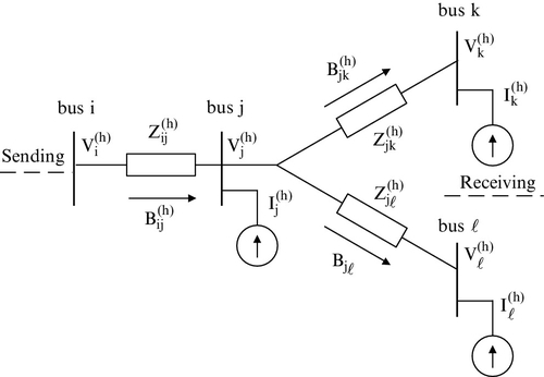
It can be seen that the relationship between branch currents and harmonic (injection) currents of a radial feeder can be calculated by summing the injection currents from the receiving bus toward the sending bus of the feeder. The general form of the harmonic currents can be expressed as

On the other hand, the relationship between branch currents and bus voltages can be shown to be

where Z(h) is the equivalent impedance of the line section at the hth harmonic frequency.
It is evident for a radial distribution system that if branch currents have been calculated, then the bus voltages can be easily determined from
The bus voltages can be obtained by calculating the voltage from the sending bus forward to the receiving bus of the feeder. Power system components are adjusted for each harmonic order.
7.5.3 Modified Fast Decoupled Harmonic Power Flow
This method extends and generalizes the conventional fast decoupled (fundamental) power flow algorithm to accommodate harmonic sources [20]. The reduced and decoupled features of the fast decoupled algorithm is explored for the harmonic power flow application. A mathematical nonlinear model is integrated into an existing fast decoupled power flow program. This method allows separate modeling of nonlinear loads and subsequently integrating them in the main algorithm without substantially increasing computation time.
The hth harmonic bus injection current vector is defined as
where Y(h) is the hth harmonic admittance matrix. The injected current at any bus p is given by

This equation provides the change of voltage magnitude and phase angle for each harmonic as a result of the injected currents.
The problem is then solved by the Newton–Raphson method. The current injected by a nonlinear load is assumed to be constant throughout the iteration and is used to modify the solution of voltage amplitudes and angles without reinverting the Jacobian matrix. At the end of each iteration, the device parameters are adjusted to reflect the new voltage magnitudes and phase angles. The harmonic currents and injected power are then reevaluated and the process is repeated until convergence is achieved.
7.5.4 Fuzzy Harmonic Power Flow
All elements of Eq. 7-139 are complex valued. Therefore, it can be reformulated as [13]

where Vr(h), Vi(h), Ir(h), and Ii(h) are the real and imaginary parts of the hth harmonic voltage and current, respectively. ψ(h) is a 2n × 2n matrix restructured from Y(h) and n is the bus number.
Fuzzy set theory is employed to represent the injection harmonic currents. For an n bus distribution system the solution is obtained by solving a set of 4n × 4n linear equations. The fuzzy solution for both harmonic magnitudes and phase angles can be individually expressed by two explicit linear equations. The solutions for any harmonic level can be easily obtained from these equations.
Harmonic sources are represented as (voltage-independent) current sources. Because harmonic penetration is a steady-state phenomenon, monitoring harmonics requires a long period of time for accurate measurements. It can be shown that the value of the harmonic currents at a bus is most likely near the center of a monitored range. Therefore, it is suitable to model the harmonic current source with a triangle fuzzy number, denoted by Ĩh. With a proper fuzzy model, the new fuzzy harmonic power flow equations can be expressed in the following form [13]:

Note that ψ(h) is a constant whereas the harmonic voltages ![]() and
and ![]() are fuzzy numbers.
are fuzzy numbers.
An arbitrary fuzzy number can be represented by an ordered pair of functions (umin (r), umax (r)), 0 ≤ r ≤ 1, which meet the following conditions:
• umin(r) is a bounded left continuous nondecreasing function over [0,1].
• umax(r) is a bounded right continuous nonincreasing function over [0,1].
• uman(r) ≤ umax(r), 0 ≤ r ≤ 1.
The fuzzy harmonic power flow can then be expressed as follows [13]:

where ψ11 contains the positive entries of [ψ], ψ12 represents the absolute values of the negative entries of [ψ], and [ψ] = ψ11 – ψ12; moreover ψ12 = ψ21 and ψ11 = ψ22. Equation 7-143 is linear and can then be uniquely solved for ![]() if and only if the matrix
if and only if the matrix ![]() is nonsingular.
is nonsingular.
7.5.5 Probabilistic Harmonic Power Flow
Unavoidable uncertainties in a power system affect the input data of the modeling for the evaluation of voltage and current harmonics caused by nonlinear loads. These uncertainties are mainly due to time variations of linear load demands, network configurations, and operating modes of nonlinear loads. The variations have a random character and, therefore, are expressed using the probabilistic method. The models available for evaluating voltage distortion are
• Direct method, in which the probability functions of harmonic voltages are calculated for assigned probability functions of harmonic currents injected by nonlinear loads.
• Integrated method, in which the probability functions of the voltage and current harmonics are calculated together by properly taking into account the interactions between voltage distortions and harmonic currents.
The probabilistic method is employed for harmonic power flow analysis to describe the interactions between the supply voltage distortions and the injected harmonic currents. It transfers the deterministic approach, which is based on the solution of a nonlinear equation system, to the field of probability.
To reduce the computational effort and to overcome the convergence problem, this method linearizes the nonlinear equation describing the steady-state behavior around an expected value region. Then, the first-order approximations are used to directly establish the means and covariance matrix of the output probability density function, starting from knowledge of the means and covariance matrix of the input probability density functions.
The following vector is defined as an input parameter (the values of the vector are kept fixed and assigned as input data [21,22]):
where T1 includes the active generator power at fundamental frequency (with the exception of the slack), T2 includes the active and reactive linear load powers at fundamental frequency and the total active and apparent nonlinear load powers, and T3 represents the generator voltage magnitudes. In all cases, some input parameters may be affected by uncertainties; hence, a probabilistic approach is adopted.
Every probabilistic formulation requires, first, the statistical characterization of the input data and, second, the evaluation of the statistical features of the output variables of interest. The statistical characterization of the input data consists of checking
(i) which components of vector Ta have to be considered as random and which ones can be kept fixed, and
(ii) what are the statistical features to characterize the randomness of the variables identified in step (i).
The most realistic approach to solve the problem is to refer to past experience, looking at both available historical data collections and technical knowledge of the electrical power system under study. According to (i), the generator voltage magnitudes can be considered deterministic if the set points of the regulator are not deliberately changed. With regard to (ii), the random nature, which appears in T1 and T2, is applied. A probabilistic method can be used to evaluate the statistical features of the output variable and may be based on the linearization around an expected value region of the nonlinear equation. The change of active and reactive linear loads is assumed to be Gaussian (normally distributed).
A probabilistic steady-state analysis of a harmonic power flow can be performed by either iterative probabilistic methods (e.g., Monte Carlo) or by analytical approaches. Iterative probabilistic procedures require knowledge of probability density functions of the input variables; for every random input data, a value is generated according to its proper probability density function. According to the generated input values, the operating steady-state conditions of the harmonic power flow are evaluated by solving the nonlinear equations by means of an iterative numerical method. Once convergence has been achieved, the state of the power system is completely known and the values of all the variables of interest are stored. The procedure is repeated to achieve a good estimate of probability of the output variables according to the stated accuracy. Unfortunately, iterative probabilistic procedures require a high computational effort.
An analytical approach is employed to linearize the nonlinear equations describing steady-state behavior of the power system around an expected value region. As a result, it offers a faster solution than the iterative probabilistic method. To evaluate the statistical procedure, the harmonic power flow equation is expressed as [21,22]
where N and Tb are the output and input random vector variables, respectively. Let the vector μ(Tb) be the expected values of Tb. Using μ(Tb) as input data for the deterministic power flow calculation results in vector No as solutions:
Linearizing the equation around the point No results in
where
J is the Jacobian matrix. Once the statistical features of the random output vector N are known, the statistics of other variables on which it depends can also be evaluated.
The use of a proper linearized approach allows a drastic reduction of computational effort because the computation required practically consists of the solution of only one deterministic harmonic power flow. Since the harmonic power flow equations are linearized around an expected value of the input vector, any movement away from this region produces an error. The errors can grow with the variance of the input random vector components, with the entity linked to the nonlinear behavior of the equation system.
7.5.6 Modular Harmonic Power Flow
The coupled harmonic power flow calculation (Section 7.4) is established by directly involving nonlinear loads as integral parts of the solution. This makes the calculation complicated. The procedure can be simplified by detaching nonlinear device models from the main program [9,11,14,23]. As most nonlinear devices can be represented by harmonic sources, detaching their models is relatively simple, and due to the iterative nature of the solution, this representation does not limit the accuracy of the results.
In modular approaches, nonlinear loads are included within the harmonic power flow as black boxes. In a black box each node has two quantities: the nodal voltage and the injected current. One quantity is specified and used to calculate the other (unknown) quantity. The procedure involves the solution of the harmonic bus voltages and using them to compute harmonic current penetration, which is then used to obtain (updated) harmonic bus voltages.
The harmonic modeling of a nonlinear load can be obtained by either a direct or an iterative approach [11,23]. The Newton method may be employed to achieve the solution. For the nonlinear buses, the mismatches are the difference between the calculated nodal values and the transferred values from the nonlinear device models. This formulation simplifies the calculation of the mismatch vector and Jacobian matrix.
The exact modeling of complex components (e.g., nonlinear loads) is carried out individually in the time domain for that particular component using the best-suited method. The calculations are performed in a modular fashion and separately for each component. The components are then assembled via a systemwide harmonic matrix that enables the bus voltages to be corrected so that the current mismatches ΔI at all nodes are iteratively forced to zero.
The modular harmonic power flow (MHPF) is performed iteratively. Each step consists of two stages:
(i) Updating the periodic steady state of the individual components (black boxes) using voltage corrections from stage (ii). The inputs to a component are the voltages at its terminals and the outputs are the terminal currents. This stage provides accurate outputs for the given inputs. The initial input voltages (at the first iteration) are usually obtained from the fundamental power flow algorithm.
(ii) Calculation of voltage corrections for stage (i). The currents obtained from stage (i) are combined for buses with adjacent components into the current mismatch ΔI, which are expressed in the harmonic domain. These become injections into a systemwide incremental harmonic admittance matrix Ybus, calculated in advance from such matrices for all individual components. The following equation is then solved for ΔV to be used in stage (i) to update all bus voltages:
The approach is modular in stage (i), but at stage (ii) the voltage correction ΔV is calculated globally for the entire system. The main procedures of the MHPF algorithm are
• A fundamental power flow algorithm is used to obtain initial voltages at all nodes.
• The incremental harmonic admittance matrix Ybus is identified. This is first done separately for each component (black box) and then the systemwide Ybus matrix is assembled.
• Currents and their mismatches ΔI are obtained for each node.
• ΔI and Ybus are used to obtain ΔV (Eq. 7-150) and the nodal voltages are finally updated for the next iteration.
The modular approach facilitates the development of new component models and the formation of a wide range of system configurations. It is also appropriate for an unbalanced system with asymmetric loads. In practice some power quality problems relate to uncharacteristic harmonic frequencies resulting from nonlinear loads and/or system asymmetries and thus requiring three-phase harmonic simulation. The solutions of MHPF algorithms are reported to be accurate as compared with those generated by the conventional (nonmodular) HPF. The computing times depend of the required accuracy of the solution at harmonic frequencies and the maximum order of harmonics.
7.5.7 Application Example 7.19: Accuracy of Decoupled Harmonic Power Flow
Apply the coupled (Section 7.4) and decoupled (Section 7.5.1) harmonic power flow algorithm to the distorted 18-bus system of Fig. E7.19.1 and compare simulation results including the fundamental and rms (including harmonics) voltages, distortion factor, and THDv. The nonlinear load (installed at bus 5) is a 3 MW, 5 MVAr six-pulse converter. Line and load parameters are provided in [29]. For the DHPF calculations, the converter may be modeled with harmonic current sources (Table E7.19.1).

Table E7.19.1
Magnitude of Harmonic Currents (as a Percentage of the Fundamental) Used to Model Six-Pulse Convertersa
| Harmonic order | Magnitude (%) | Harmonic order | Magnitude (%) | Harmonic order | Magnitude (%) |
| 1 | 100 | 19 | 2.4 | 37 | 0.5 |
| 5 | 19.1 | 23 | 1.2 | 41 | 0.5 |
| 7 | 13.1 | 25 | 0.8 | 43 | 0.5 |
| 11 | 7.2 | 29 | 0.2 | 47 | 0.4 |
| 13 | 5.6 | 31 | 0.2 | 49 | 0.4 |
| 17 | 3.3 | 35 | 0.4 |

a All harmonic phase angles are assumed to be zero.
Solution to Application Example 7.19
The Newton-based HPF (e.g., using an accurate converter model that includes harmonic couplings [5,6]) and the DHPF (modeling the converter with harmonic current sources of Table E7.19.1) are applied to the 18 bus system. Simulation results are compared in Table E7.19.2. Small levels of the maximum and average deviations (last two rows of Table E7.19.2) show the acceptable accuracy of the decoupled approach.
Table E7.19.2
Comparison of Simulation Results for the 18 Bus System (Fig. E7.19.1) Using Coupled (Section 7.4) and Decoupled (Section 7.5.1) Harmonic Power Flow
| bus | fundamental voltage (pu) | rms voltage (pu) | distortion factor D (%) | THD of voltage (%) | ||||
| decoupled HPF | coupled HPF | decoupled HPF | coupled HPF | decoupled HPF | coupled HPF | decoupled HPF | coupled HPF | |
| 1 | 1.0545 | 1.0545 | 1.0549 | 1.0548 | 0.9996 | 0.9997 | 2.7159 | 2.3828 |
| 2 | 1.0511 | 1.0510 | 1.0516 | 1.0516 | 0.9995 | 0.9995 | 3.1353 | 3.1942 |
| 3 | 1.0456 | 1.0455 | 1.0463 | 1.0465 | 0.9993 | 0.9991 | 3.6591 | 4.2593 |
| 4 | 1.0425 | 1.0424 | 1.0433 | 1.0436 | 0.9992 | 0.9989 | 3.9386 | 4.7737 |
| 5 | 1.0359 | 1.0358 | 1.0370 | 1.0377 | 0.9989 | 0.9982 | 4.7701 | 6.0515 |
| 6 | 1.0348 | 1.0347 | 1.0360 | 1.0367 | 0.9988 | 0.9981 | 4.8692 | 6.1886 |
| 7 | 1.0326 | 1.0325 | 1.0339 | 1.0347 | 0.9987 | 0.9979 | 5.1238 | 6.5404 |
| 8 | 1.0268 | 1.0267 | 1.0281 | 1.0289 | 0.9987 | 0.9978 | 5.1528 | 6.5775 |
| 9 | 1.0496 | 1.0496 | 1.0501 | 1.0501 | 0.9995 | 0.9995 | 3.1397 | 3.1985 |
| 20 | 1.0505 | 1.0504 | 1.0509 | 1.0509 | 0.9996 | 0.9996 | 2.9329 | 2.9248 |
| 21 | 1.0496 | 1.0495 | 1.0505 | 1.0506 | 0.9991 | 0.9990 | 4.1782 | 4.4609 |
| 22 | 1.0479 | 1.0479 | 1.0488 | 1.0489 | 0.9991 | 0.9990 | 4.1847 | 4.4682 |
| 23 | 1.0451 | 1.0451 | 1.0474 | 1.0477 | 0.9978 | 0.9974 | 6.6676 | 7.1620 |
| 24 | 1.0485 | 1.0485 | 1.0519 | 1.0523 | 0.9968 | 0.9964 | 7.9886 | 8.4865 |
| 25 | 1.0419 | 1.0418 | 1.0449 | 1.0452 | 0.9971 | 0.9967 | 7.6002 | 8.1187 |
| 26 | 1.0415 | 1.0414 | 1.0445 | 1.0449 | 0.9971 | 0.9967 | 7.6029 | 8.1220 |
| 50 | 1.0501 | 1.0501 | 1.0501 | 1.0501 | 1.0000 | 1.0000 | 0.2482 | 0.1217 |
| 51 | 1.0500 | 1.0500 | 1.0500 | 1.0500 | 1.0000 | 1.0000 | 0.2482 | 0.0035 |
| MDa | 0.0097 | - | 0.0778 | - | 0.0009 | - | 1.42473 | - |
| ADb | 0.0059 | - | 0.0278 | - | 0.0003 | - | 0.57242 | - |

a Maximum Deviation with respect to the coupled HPF (%).
b Average Deviation with respect to the coupled HPF (%).
7.6 Summary
After an overview of the interconnected power system and its components, power system matrices are introduced, in particular the bus admittance matrix. Bus-building algorithms are explained, and the concepts of singularity and nonsingularity of matrices and their physical interpretation with respect to power systems are discussed. After a brief review of matrix solution techniques under the aspects of matrix sparsity, the fundamental power flow technique is used to explain the Newton–Raphson solution method. The harmonic power flow problem is firmly grounded on the fundamental power flow: additional circuit conditions are introduced for the harmonic power flow problem.
Numerous application examples detail for the fundamental power flow analysis the bus-building algorithm, matrix manipulations – such as multiplication and triangular factorization – formation of the Jacobian, definition of mismatch vector, and the recursive application of the Newton–Raphson algorithm. Similarly, the application examples cover the step-by-step approach for one iteration of the harmonic Newton-type solution method. The chapter concludes with a classification of existing power flow techniques.
7.7 Problems
Problem 7.1: Determination of Admittance Matrices 
a) Determine the bus admittance matrices ![]() referenced to ground for Fig. P7.1a,b,c,d.
referenced to ground for Fig. P7.1a,b,c,d.


b) The system of Fig. P7.1d has no admittance connected from any one of the buses to ground. Show that its admittance matrix is singular.
Problem 7.2: Establishing the Table of Factors
For the real matrix Ā

b) Solve

for the vector ![]() .
.
Problem 7.3: Voltage Control via Inductive Load (e.g., Reactors)
Apply the Newton–Raphson load flow analysis technique to the three-bus power system of Fig. P7.3, provided switch S1 is closed and switch S2 is open.

a) Find the fundamental bus admittance matrix in polar form.
b) Assume that bus 1 is the swing (slack) bus and buses 2 and 3 are PQ buses. Make an initial guess for the bus voltage vector ![]() and evaluate the initial mismatch power
and evaluate the initial mismatch power ![]()
c) Find the Jacobian ![]() for this power system configuration and compute the bus voltage correction vector
for this power system configuration and compute the bus voltage correction vector ![]()
d) Update the bus voltage vector ![]() and recompute the updated mismatch power vector
and recompute the updated mismatch power vector ![]()
Problem 7.4: Voltage Control via Capacitive Load (e.g., Capacitors)
Repeat Problem 7.3 for the condition when switch S1 is open and switch S2 is closed.
Problem 7.5: Fundamental Power Flow Exploiting the Symmetry of a Power System
Apply to the two-bus system of Fig. P7.5 the Newton–Raphson load flow analysis technique.

a) Simplify the two-bus system.
b) Find the fundamental bus admittance matrix in polar form.
c) Assume that bus 1 is the swing (slack) bus, and bus 2 is a PQ bus. Make an initial guess for the voltage vector ![]() and evaluate the initial mismatch power
and evaluate the initial mismatch power ![]()
d) Find the Jacobian matrix ![]() for this power system configuration and compute the bus voltage correction vector
for this power system configuration and compute the bus voltage correction vector ![]()
e) Update the bus voltage vector ![]() and recompute the updated mismatch power vector
and recompute the updated mismatch power vector ![]()
Problem 7.6: Fundamental Power Flow in a Weak Power System
The power system of Fig. P7.6 represents a weak feeder as it occurs in distributed generation (DG) with wind-power plants and photovoltaic plants as power sources. All impedances are in pu and the base apparent power is Sbase = 10 MVA.

a) Compute the fundamental admittance matrix for this system.
b) Assuming bus 1 is the swing bus (δ1 = 0 and ![]() = 1.0 pu) then we can make an initial guess for bus voltage vector
= 1.0 pu) then we can make an initial guess for bus voltage vector ![]() = (δ2,
= (δ2, ![]() , δ3,
, δ3, ![]() , δ4,
, δ4, ![]() )t = (0, 1, 0, 1, 0, 1)t. Note, the superscript 0 means initial guess. Compute the mismatch power vector for this initial condition.
)t = (0, 1, 0, 1, 0, 1)t. Note, the superscript 0 means initial guess. Compute the mismatch power vector for this initial condition.
c) Compute the Jacobian matrix.
d) Compute the inverse of the Jacobian matrix.
e) Compute the correction voltage vector ![]() update the mismatch power vector, and check the convergence of the load flow algorithm (using a convergence tolerance of 0.0001).
update the mismatch power vector, and check the convergence of the load flow algorithm (using a convergence tolerance of 0.0001).
Problem 7.7: Harmonic Power Flow in a Weak Power System with One Nonlinear Bus and One Set of Harmonic Nonlinear Device Currents
The power system of Fig. P7.7 represents a weak feeder as it occurs in distributed generation (DG) with wind-power plants and photovoltaic plants as power sources. All impedances are in pu and the base apparent power is Sbase = 10 MVA. The harmonic v-i characteristic of the nonlinear load at bus 4 (referred to the voltage at bus 4) is given as

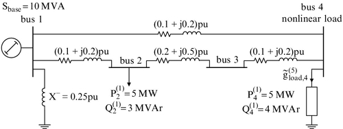
It will be assumed that the voltage at the swing bus (bus 1) is ![]() = 1.00 pu and
= 1.00 pu and ![]() rad. The fundamental power flow can be based on Fig. P7.6. For the 5th harmonic the synchronous machine impedance Z1 is replaced by the (subtransient) impedance Z2 ≈ jX− = j0.25 pu at 60 Hz. In this case the subtransient reactance has been chosen to be that of a synchronous generator in order to approximate bus 1 as a weak bus.
rad. The fundamental power flow can be based on Fig. P7.6. For the 5th harmonic the synchronous machine impedance Z1 is replaced by the (subtransient) impedance Z2 ≈ jX− = j0.25 pu at 60 Hz. In this case the subtransient reactance has been chosen to be that of a synchronous generator in order to approximate bus 1 as a weak bus.
a) Compute the fundamental and 5th harmonic admittance matrices.
b) Assume an initial value for the bus vector Ū0 and compute the fundamental and the 5th harmonic currents injected into the system by the nonlinear load.
c) Evaluate the mismatch vector.
d) Evaluate the Jacobian matrix.
e) Evaluate the correction vector ΔUo.
f) Update the mismatch vector and comment on the convergence of the harmonic load flow.