
2.7 Grounding
Proper power system grounding is very essential for personnel safety, equipment protection, and power continuity to electrical loads. Special attention should be given to grounding location and means for minimizing circulating ground currents, as well as ground-fault sensing. Electrical power systems require two types of grounding, namely, system grounding and equipment grounding; each has its own functions [55]. The IEEE Green Book, IEEE Recommended Practice for Grounding of Industrial and Commercial Power Systems, ANSI/IEEE C114.1, Std.142, is the authoritative reference on grounding techniques [56].
2.7.1 System Grounding
System and circuit conductor grounding is an intentional connection between the electric system conductors and grounding electrodes that provides an effective connection to ground (earth). The basic objectives being sought are to
• limit overvoltages due to lightning,
• limit line surges, or unintentional contact with high-voltage lines,
• stabilize the voltage to ground during normal operation, and
• facilitate overcurrent device operation in case of ground faults.
2.7.1.1 Factors Influencing Choice of Grounded or Ungrounded System
Whether or not to ground an electrical system is a question that must be faced sometime by most engineers charged with planning electrical distribution. A decision in favor of a grounded system leads then to the question of how to ground.
Definitions
• Solidly grounded: no intentional grounding impedance.
• Effectively grounded: grounded through a grounding connection of sufficiently low impedance (inherent or intentionally added or both) such that ground faults that may occur cannot build up voltages in excess of limits established for apparatus, circuits, or systems so grounded. R0 < X1, X0 ≤ 3X1, where X1 is the leakage reactance, and X0 and R0 are the grounding reactance and resistance, respectively.
• Reactance grounded: X0 ≤ 10X1.
• Resistance grounded: R0 ≥ 2X0.
• High-resistance grounded: ground fault up to 10 A is permitted.
• Grounded for serving line-to-neutral loads: Z0 ≤ Z1.
• Ungrounded: no intentional system grounding connection.
Service Continuity
For many years a great number of industrial plant distribution systems have been operated ungrounded (Fig. 2.45) at various voltage levels. In most cases this has been done with the thought of gaining an additional degree of service continuity. The fact that any one contact occurring between one phase of the system and ground is unlikely to cause an immediate outage to any load may represent an advantage in many plants (e.g., submarines), varying in its importance according to the type of plant.

Grounded Systems
In most cases systems are designed so that circuit protective devices will remove a faulty circuit from the system regardless of the type of fault. A phase-to-ground fault generally results in the immediate isolation of the faulted circuit with the attendant outage of the loads on that circuit (Fig. 2.46). However, experience has shown in a number of systems that greater service continuity may be obtained with grounded-neutral than with ungrounded-neutral systems.

Multiple Faults to Ground
Although a ground fault on one phase of an ungrounded system generally does not cause a service interruption, the occurrence of a second ground fault on a different phase before the first fault is cleared does result in an outage (Fig. 2.47). If both faults are on the same feeder, that feeder will be opened. If the second fault is on a different feeder, both feeders may be deenergized.

The longer a ground fault is allowed to remain on an ungrounded system, the greater is the likelihood of a second ground fault occurring on another phase resulting in an outage. The advantage of an ungrounded system in not immediately dropping load upon the occurrence of a ground fault may be largely destroyed by the practice of ignoring a ground fault until a second one occurs and repairs are required to restore service. With an ungrounded system it is extremely important that an organized maintenance program be provided so that first ground fault is located and removed as soon as possible after its occurrence.
Safety
Many of the hazards to personnel and property existing in some industrial electrical systems are the result of poor or nonexisting grounding of electrical equipment and metallic structures. Although the subject of equipment grounding is treated in the next section, it is important to note that regardless of whether or not the system is grounded, safety considerations require thorough grounding of equipment and structures.
Proper grounding of a low-voltage (600 V or less) distribution system may result in less likelihood of accidents to personnel than leaving the system supposedly ungrounded. The knowledge that a circuit is grounded generally will result in greater care on the part of the workman.
It is erroneous to believe that in an ungrounded system a person may contact an energized phase conductor without personal hazard. As Fig. 2.48 shows, an ungrounded system with balanced phase-to-ground capacitance has rated line-to-neutral voltages existing between any phase conductor and ground. To accidentally or intentionally contact such a conductor may present a serious, perhaps lethal shock hazard in most instances.

During the time a ground fault remains on one phase of an ungrounded system, personnel contacting one of the other phases and ground are subjected to a voltage 1.73 (that is, ![]() ) times that which would be experienced on a solidly neutral-grounded system. The voltage pattern would be the same as the case shown in Fig. 2.48c.
) times that which would be experienced on a solidly neutral-grounded system. The voltage pattern would be the same as the case shown in Fig. 2.48c.
Power System Overvoltages
Some of the more common sources of overvoltages on a power system are the following:
• lightning (see Application Examples 2.9 and 2.10),
• switching surges,
• capacitor switching,
• static,
• contact with high-voltage system,
• line-to-ground faults,
• resonant conditions, and
• restriking ground faults.
Lightning
Most industrial systems are effectively shielded against direct lightning strikes (Fig. 2.49). Many circuits are either underground in ducts or within grounded metal conduits or raceways. Even open-wire circuits are often shielded by adjacent metallic structures and buildings. Large arresters applied at the incoming service limit the surge voltages within the plant resulting from lightning strikes to the exposed service lines. Other arrester applications may be necessary within the plant to protect low impulse strength devices such as rotating machines and computers.

Switching Surges
Normal switching operation in the system (e.g., capacitor switching) can cause overvoltages. These are generally not more than three times the normal voltage and of short duration.
2.7.1.2 Application Example 2.9: Propagation of a Surge through a Distribution Feeder with an Insulator Flashover
This example illustrates the performance of a transmission system when the current of a lightning strike is large enough to cause flashover of tower insulator strings [57]. A lightning strike with the rise time τ1 = 1.0 μsec, the fall time τ2 = 5.0 μs, and the peak magnitude of current waveform I0 = 15.4 kA strikes a 138 kV transmission line at node 1 (see Fig. E2.9.1). The span lengths of this transmission line are nonuniform and are given by NL (normalized length). Both ends of the transmission line are terminated by Z0 = 300 Ω.

The transmission line has steel towers with 10 porcelain insulators. The tower-surge impedance consists of a 20 Ω resistance in series with 20 μH of inductance. The model used to simulate the first two insulators is shown in Fig. E2.9.1. Note that the transmission line can be simulated by the PSpice (lossless) transmission line model T, where Z0 = 300 Ω, f = 60 Hz, and NL as indicated in Fig. E2.9.1. The current-controlled switch can be simulated by W, where ION = 1 A.
a) Calculate the four span lengths in meters.
b) Calculate (using PSpice) and plot the transmission line voltage (in MV) as a function of time (in μs) at the point of strike, at the first insulator, and at the second insulator.
Solution to Application Example 2.9
a) The normalized length of a distance traveled by a wave (e.g., span) NL is a function of the frequency f, the span length l, and the speed of light c = 2.99792 · 108 m/s [58]: ![]() or the length of a span is
or the length of a span is ![]() . The time to travel the distance NL · λ, where λ is the wavelength, is
. The time to travel the distance NL · λ, where λ is the wavelength, is ![]() .
.
Length of span #1: l1 = 2500 m, length of span #2: l2 = 500 m, length of span #3: l3 = 1000 m, length of span #4: l4 = 1000 m.
b) The PSpice program is listed in Table E2.9.1. One obtains the results of Figs. E2.9.2 and E2.9.3.
Table E2.9.1
PSpice Program Codes for Propagation of a Surge through a Distribution Feeder with an Insulator Flashover (Application Example 2.9)
| *Lightning performance of a transmission line *Insulator flashover *lightning current source i1 1 0 exp(0 15.4k 0 1.0u 2.0111u 5u) *span#1 t1 1 0 3 0 z0=300 f=60 NL=100u *insulator #1 d1 13 3 dmod L1 13 53 20u vs1 23 53 dc 0 w1 23 33 vs1 wmod1 rvs1 33 43 20 vd1 0 43 3700k rft1 23 0 20 *span#2 t2 3 0 5 0 z0=300 f=60 NL=200u *insulator#2 d2 15 5 dmod L2 15 55 20u vs2 25 55 dc 0 w2 25 35 vs2 wmod1 rvs2 35 45 20 vd2 0 45 3700k rft2 25 0 20 *span#3 t3 5 0 7 0 z0=300 f=60 NL=200u *z RL3 7 0 300 *span#4 t4 1 0 9 0 z0=300 f=60 NL=500u *z RL4 9 0 300 .model dmod d(is=1e-14) .model wmod1 iswitch (ron=1 roff=1e6 ion=1 ioff=1.01) .tran 0.1u 20u 0 0.05u .options chgtol=2u abstol=2u vntol=2u .options ITL4=200 ITL5=0 LIMPTS=100000 reltol=0.001 .probe .print tran V(1) V(3) V(5) .end |


2.7.1.3 Application Example 2.10: Lightning Arrester Operation
This problem illustrates the performance of a lightning arrester [57]. The same basic parameters as for the lightning strike employed in Application Example 2.9 are used in this example. The only changes are in the value of I0 (in this problem a value of 7.44 kA is assumed) and in the voltage of the second lightning arrester (VD2 = 600 kV). This value is small enough that flashover of the insulator string will not occur; however, it is large enough to cause the lightning arrester to operate due to VD2 = 600 kV. The system being simulated is shown in Fig. E2.10.1.

a) Calculate and plot the transmission line voltage (in MV) as a function of time (in μs) at the point of strike, at the insulator, and at the lightning arrester.
b) Calculate and plot the currents at the point of strike, at the insulator, and at the lightning arrester (in kA) as a function of time (in μs).
Solution to Application Example 2.10
a) Calculations are performed using PSpice, and the plots of the transmission line voltage (in MV) as a function of time (in μs) at the point of strike, at the insulator, and at the lightning arrester are shown in Figs. E2.10.2 and E2.10.3. The PSpice program is listed in Table E2.10.1.


Table E2.10.1
PSpice Program Codes for Lightning Arrester Operation (Application Example 2.10)
*Lightning performance of a transmission line
*lightning arrester operation
*lightning current source
i1 1 0 exp(0 7.44k 0 1.0u 2.011u 5u)
*span#1
t1 1 0 3 0 z0=300 f=60 NL=100u
*insulator #1
d1 13 3 dmod
L1 13 53 20u
vs1 23 53 dc 0
w1 23 33 vs1 wmod1
rvs1 33 43 20
vd1 0 43 3700k
rft1 23 0 20
*span#2
t2 3 0 5 0 z0=300 f=60 NL=200u
*insulator#2
d2 15 5 dmod
L2 15 55 20u
vs2 25 55 dc 0
w2 25 35 vs2 wmod1
rvs2 35 45 20
vd2 0 45 600k
rft2 25 0 20
*span#3
t3 5 0 7 0 z0=300 f=60 NL=200u
*z
RL3 7 0 300
*span#4
t4 1 0 9 0 z0=300 f=60 NL=500u
*z
RL4 9 0 300
.model dmod d(is=1)
.model wmod1 iswitch (ron=1 roff=1e6 ion=0.8
+ ioff=0.3)
.tran 0.1u 30u 0 0.05u
.options chgtol=2u abstol=2u vntol=2u
.options ITL4=25 ITL5=0 LIMPTS=100000 reltol=0.001
.probe
.print tran V(1) V(3) V(5) -i(i1(t)) i(vs1) i(vs2)
.end
b) One obtains the results of Figs. E2.10.4 and E2.10.5 using the PSpice program codes of Table E2.10.1. This is a good example where the various versions of PSpice have different convergence properties similar to the Mathematica software (see Application Example 8.5).


2.7.2 Equipment Grounding
All exposed metal parts of electrical equipment (including generator frames, mounting bases, electrical instruments, and enclosures) should be bonded to a grounding electrode.
Basic Objectives
Equipment grounding, in contrast with system grounding, relates to the manner in which nonelectrical conductive material, which encloses energized conductors or is adjacent thereto, is to be interconnected and grounded. The basic objectives being sought are the following:
• to maintain a low potential difference between nearby metal members, and thereby protect people from dangerous electric-shock-voltage exposure in a certain area,
• to provide current-carrying capability, both in magnitude and duration, adequate to accept the ground-fault current permitted by the overcurrent protection system without creating a fire or explosive hazard to buildings or contents,
• to provide an effective electrical path over which ground-fault currents can flow without creating a fire or explosive hazard, and
• to contribute to superior performance of the electrical system (e.g., suppression of differential and common-mode electrical noise, discussed in Chapter 11).
Investigations have pointed out that it is important to have good electric junctions between sections of conduit or metal raceways that are used as equipment grounding paths, and to assure adequate cross-sectional areas and conductivity of these grounding paths. Where systems are solidly grounded, equipment grounding conductors are bonded to the system grounded conductor and the grounding electrode conductor at the service equipment and at the source of a separately derived system in accordance with the National Electrical Code (NEC) Article 250 [55,56].
2.7.3 Static Grounding
The British standard [59] regarding grounding states that the most common source of danger from static electricity is the retention of charge on a conductor, because virtually all the stored energy can be released in a single spark to earth or to another conductor. The accepted method of avoiding the hazard is to connect all conductors to each other and to earth via electrical paths with resistances sufficiently low to permit the relaxation of the charges. This was stated in the original British standard (1980) and is carried out worldwide [60].
Purpose of Static Grounding
The accumulation of static electricity, on materials or equipment being handled or processed by operating personnel, introduces a potentially serious hazard in any area where combustible gases, dusts, or fibers are present. The discharge of the accumulation of static electricity from an object to ground or to another ungrounded object of lower potential is often the cause of a fire or an explosion if it takes place in the presence of readily combustible materials or combustible vapor and air mixtures.
2.7.4 Connection to Earth
Resistance to Earth. The most elaborate grounding system that can be designed may prove to be inadequate unless the connection of the system to the earth is adequate and has a low resistance. It follows, therefore, that the earth connection is one of the most important parts of the whole grounding system. It is also the most difficult part to design and to obtain. The perfect connection to earth should have zero resistance, but this is impossible to obtain. Ground resistance of less than 1 Ω can be obtained, although this low resistance may not be necessary in many cases. Since the desired resistance varies inversely with the fault current to ground, the larger the fault current, the lower must be the resistance [61,62]. Figure 2.50a illustrates the deformation of grounding conductor due to large lightning currents.

2.7.5 Calculation of Magnetic Forces
Considerable work [63,64] has been done concerning the calculation of electromagnetic forces based on closed-form analysis. These methods can be applied to simple geometric configurations only. In many engineering applications, however, three-dimensional geometric arrangements must be analyzed. Based on the theory developed by Lawrenson [65] filamentary conductor configurations can be analyzed. Figures 2.50a,b illustrate the force density distribution for a filamentary 90° bend at a current of I = 100 kA. Three-dimensional arrangements are investigated in [66]. Force calculations based on the so-called Maxwell stress are discussed in Chapter 4.
2.8 Measurement of derating of three-phase transformers
Measuring the real and apparent power derating of three-phase transformers is desirable because additional losses due to power quality problems (e.g., harmonics, DC excitation) can be readily limited before any significant damage due to additional temperature rises occurs [8,9]. Measuring transformer losses from the input power minus the output power in real time is inaccurate because the losses are the difference of two large values; this indirect approach results in maximum errors in the losses of more than 60% for high-efficiency (η > 98%) transformers [7]. The usually employed indirect method consisting of no-load (iron-core loss) and short-circuit (copper loss) tests [67] cannot be performed online while the transformer is partially or fully loaded. IEEE Recommended Practice C57.110 computes the transformer derating based on Rh for various harmonics h, which is derived from the DC winding resistance and the rated load loss [14]. Kelly et al. [68] describe an improved measuring technique of the equivalent effective resistance RT as a function of frequency f of single-phase transformers, which allows the direct calculation of transformer loss at harmonic frequencies from f = 10 Hz up to 100 kHz. This equivalent effective resistance takes into account the total losses of the transformer: the copper losses plus the iron-core losses. Based on the fact that the iron-core losses do not depend on harmonic currents, but depend on harmonic voltages (amplitudes and phase shifts) [69], the total losses determined by [68] are not accurate. In addition, temperature-dependent operating conditions cannot be considered in [68]. Mocci [70] and Arri et al. [71] present an analog measurement circuit to directly measure the total losses for single- and ungrounded three-phase transformers. However, employment of many potential transformers (PTs) and current transformers (CTs) in the three-phase transformer measuring circuits [71] decreases the measurement accuracy.
This section presents a direct method for measuring the derating of three-phase transformers while transformers are operating at any load and any arbitrary conditions. The measuring circuit is based on PTs, CTs, shunts, voltage dividers or Hall sensors [72], A/D converter, and computer (microprocessor). Using a computer-aided testing (CAT) program [7,73], losses, efficiency, harmonics, derating, and wave shapes of all voltages and currents can be monitored within a fraction of a second. The maximum errors in the losses are acceptably small and depend mainly on the accuracy of the sensors used.
2.8.1 Approach
2.8.1.1 Three-Phase Transformers in Δ–Δ or Y–Y Ungrounded Connection
For Δ–Δ or ungrounded Y–Y connected three-phase transformers (see Figs. 2.51 and 2.52 for using shunts, voltage dividers, and optocouplers), one obtains with the application of the two-wattmeter method at the input and output terminals by inspection:


The term ![]() represents the instantaneous iron-core loss, and
represents the instantaneous iron-core loss, and ![]() is the instantaneous copper loss.
is the instantaneous copper loss.
2.8.1.2 Three-Phase Transformers in Δ–Y Connection
Figure 2.53 illustrates the application of the digital data-acquisition method to a Δ–Y connected transformer bank.

For ungrounded Δ–Y connected three-phase transformers, the currents of the Y side must be referred to the line currents of the Δ side, as shown in Fig. 2.53. The loss of the transformer is given by


where iAl and iBl are input line currents of phases A and B, respectively; ![]() and
and ![]() are the two-wattmeter secondary currents; van′ and vcn′ are the output line-to-neutral voltages of phases a and c, respectively.
are the two-wattmeter secondary currents; van′ and vcn′ are the output line-to-neutral voltages of phases a and c, respectively.
Because the neutral of the Y-connected secondary winding (N) is not accessible, the secondary phase voltages are measured and referred to the neutral n of the Y-connected PTs (see Fig. 2.53). This does not affect the accuracy of loss measurement, which can be demonstrated below. The output power is

where N denotes the neutral of the Y-connected secondary winding. Because ![]() = 0, the measured output power referred to the neutral n of PTs is the same as that referred to the neutral N of the secondary winding.
= 0, the measured output power referred to the neutral n of PTs is the same as that referred to the neutral N of the secondary winding.
2.8.1.3 Accuracy Requirements for Instruments
The efficiencies of high-power electrical apparatus such as single- and three-phase transformers in the kVA and MVA ranges are 97% or higher. For a 15 kVA three-phase transformer with an efficiency of 97.02% at rated operation, the total losses are PLoss = 409.3 W, copper and iron-core losses Pcu = 177.1 W and Pfe = 232.2 W at VL-L = 234.2 V and IL = 32.4 A, respectively, as listed in Table 2.7a.
The determination of the losses from voltage and current differences as described in Fig. 2.51 – where differences are calibrated – greatly reduces the maximum error in the loss measurement. The series voltage drop and exciting current at rated operation referred to the primary of the 15 kVA, 240 V/240 V three-phase transformer are (vAC – vac‘) = 3.56 V, (iA – ia‘) = 2.93 A, respectively (Table 2.7a). The instruments and their error limits are listed in Table 2.1. In Table 2.1, vAC, vAC – vacʹ, iA – iaʹ, and iaʹ stand for the relevant calibrated voltmeters and ammeters. Because all voltage and current signals are sampled via PTs, CTs (or optocouplers), and current shunts, the error limits for all instruments are equal to the product of the actually measured values and their relative error limits, instead of full-scale errors, as shown in Table 2.1. All error limits are referred to the meter side.
Table 2.1
Instruments and Their Error Limits for Figs. 2.51 and 2.52
| Instrument (Fig. 2.51) | Instrument (Fig. 2.52) | Rating | Error limits |
| PT1 | VDA | 240 V/240 V | |
| PT2 | VDa | 240 V/240 V | |
| CT1 | SHA | 30 A/5 A | |
| CT2 | SHa | 30 A/5 A | |
| vAC | vAC | 300 V | |
| vAC – vac′ | vAC – vac′ | 10 V | |
| iA – ia′ | iA – ia′ | 5 A | |
| ia′ | ia′ | 5 A |

In Fig. 2.52, the voltage divider (R1A, R2A) combined with an optocoupler (vAc) emulates the function of a PT without hysteresis. The optocoupler can alter the amplitude of a signal and provides isolation without affecting the phase shift of the signal as it is corrupted by PTs. The current shunt ![]() and optocouplers
and optocouplers ![]() emulate that of a CT without hysteresis and parasitic phase shift. The prime (ʹ) indicates that iaʹ is about of the same magnitude as iA; this is accomplished by adjustment of the amplifier gain(s) of the optocoupler(s). VD and SH in Table 2.1 stand for voltage divider and shunt, respectively.
emulate that of a CT without hysteresis and parasitic phase shift. The prime (ʹ) indicates that iaʹ is about of the same magnitude as iA; this is accomplished by adjustment of the amplifier gain(s) of the optocoupler(s). VD and SH in Table 2.1 stand for voltage divider and shunt, respectively.
The line-to-line voltage is measured with the maximum error of (taking into account the maximum errors of PT1 and voltmeter)

The current difference is measured with the maximum error of

Therefore, the loss component vAC (iA – ia‘) in Eq. 2-49 is measured with the maximum error of

The series voltage drop is measured with the maximum error of

The output current is measured with the maximum error of
and the loss component (vAC – vacʹ)iaʹ in Eq. 2.49 is measured with the maximum error of
Thus, the total loss is measured with the maximum error of

The above error analysis employs PTs and CTs. If these devices generate too-large errors because of hysteresis, voltage dividers (e.g., VDA) and shunts (e.g., SHA) combined with optocouplers can be used, as indicated in Fig. 2.52 [74]. A similar error analysis using shunts, dividers, and optocouplers leads to the same maximum error in the directly measured losses, provided the same standard maximum errors (0.1%) of Table 2.1 are assumed. The factor 2 in Eq. 2-58 is employed because loss components in Eq. 2-54 and Eq. 2-57 are only half of those in Eq. 2-49.
2.8.1.4 Comparison of Directly Measured Losses with Results of No-Load and Short-Circuit Tests
A computer-aided testing electrical apparatus program (CATEA) [73] is used to monitor the iron-core and copper losses of three-phase transformers. The nameplate data of the tested transformers are given in Appendixes 3.1 to 3.4. The results of the on-line measurement of the iron-core and copper losses for a Y–Y connected 9 kVA three-phase transformer (consisting of three 3 kVA single-phase transformers, Appendix 3.1) are given in Table 2.2 for sinusoidal rated line-to-line voltages of 416 V, where the direct (online) measurement data are compared with those of the indirect (separate open-circuit and short-circuit tests) method. The iron-core loss of the indirect method is larger than that of the direct method because the induced voltage of the former is larger than that of the latter. The copper loss of the indirect method is smaller than that of the direct method because the input current of the former (which is nearly the same as the output current) is smaller than that of the latter.
2.8.2 A 4.5 kVA Three-Phase Transformer Bank #1 Feeding Full-Wave Rectifier
A 4.5 kVA, 240 V/240 V, Δ–Δ connected three-phase transformer (Fig. 2.51) consisting of three single-phase transformers (bank #1, Appendix 3.2) is used to feed a full-wave diode rectifier (see Appendix 3.5) with an LC filter connected across the resistive load (see Fig. 6-5 of [75]). In Table 2.3, measured data are compared with those of linear load condition. The measured wave shapes of input voltage (vAC), exciting current (iA – iaʹ), series voltage drop (vAC – vacʹ), and output current (ia‘) of phase A are shown in Fig. 2.54a,b for linear and nonlinear load conditions. The total harmonic distortion THDi, K-factor, and harmonic components of the output current are listed in Table 2.4.
Table 2.3
Measured Data of 4.5 kVA Transformer Bank #1
| Linear load (Fig. 2.54a) | Nonlinear load (Fig. 2.54b) | |
| vAC | 237.7 Vrms | 237.7 Vrms |
| 1.10 Arms | 1.12 Arms | |
| 8.25 Vrms | 8.19 Vrms | |
| ia′ | 11.09 Arms | 10.98 Arms |
| Iron-core loss | 100.7 W | 103.9 W |
| Copper loss | 161.3 W | 157.6 W |
| Total loss | 262.0 W | 261.5 W |
| Output power | 4532 W | 4142 W |
| Efficiency | 94.55% | 94.09% |

Table 2.4
Output Current Harmonic Components, THDi, and K-Factor (Fig. 2.54b)
| ih (Arms) | ||||||
| h = 1 | h = 5 | h = 7 | h = 11 | h = 13 | THDi (%) | K |
| 10.4 | 3.55 | 0.81 | 0.77 | 0.24 | 36.34 | 4.58 |

Table 2.3 compares measured data and shows that the transformer is operated at nonlinear load with about the same losses occurring at linear load (261.3 W). With the apparent power derating definition

the derating at the nonlinear load of Table 2.3 is 99%. The real power delivered to the nonlinear load is 91.4% of that supplied at linear load.
2.8.3 A 4.5 kVA Three-Phase Transformer Bank #2 Supplying Power to Six-Step Inverter
A 4.5 kVA transformer bank #2 (Appendix 3.3) supplies power to a half-controlled six-step inverter (Appendix 3.6), which in turn powers a three-phase induction motor. The motor is controlled by adjusting the output current and frequency of the inverter. The transformer is operated at rated loss at various motor speeds. Rated loss of bank #2 is determined by a linear (resistive) load at rated operation. The iron-core and copper losses are measured separately and are listed in Table 2.5a. Measured wave shapes of input voltage, exciting current, series voltage drop, and output current of phase A are shown in Fig. 2.55a,b for linear and nonlinear conditions. The output current includes both odd and even harmonics due to the half-controlled input rectifier of the six-step inverter. Dominant harmonics of input voltage and output current are listed for different motor speeds in Table 2.5b. The total harmonic distortion of the input voltage and output current as well as the K-factor are listed in Table 2.5c for the speed conditions of Tables 2.5a and 2.5b.
Table 2.5a
Measured Iron-Core and Copper Losses of 4.5 kVA Δ–Δ Connected Transformer Bank #2 Feeding a Six-Step Inverter at Various Motor Speeds (Fig. 2.55b)
| Motor speed (%)a | Input voltage (Vrms) | Output current (Arms) | Core loss (W) | Copper loss (W) | Total loss (W) | Output power (W) |
| b | 237.8 | 11.4 | 65.7 | 154.9 | 220.6 | 4542 |
| 100 | 237.9 | 11.1 | 69.6 | 150.5 | 220.2 | 3216 |
| 90 | 238.1 | 11.5 | 62.9 | 158.8 | 221.7 | 2913 |
| 80 | 238.3 | 11.2 | 65.6 | 153.3 | 218.9 | 2398 |
| 70 | 238.3 | 11.3 | 65.7 | 154.8 | 220.4 | 2081 |
| 60 | 238.2 | 11.4 | 64.5 | 162.2 | 226.7 | 1862 |
| 50 | 238.4 | 10.8 | 69.2 | 151.3 | 220.6 | 1530 |
| 40 | 238.6 | 11.1 | 68.5 | 151.2 | 219.7 | 1308 |

a Refers to rated speed of 1145 rpm.
b Linear resistive load.

Table 2.5b
Input Voltage (in rms Volts) and Output Current (in rms Amperes) Harmonics of Phase A (Fig. 2.55a,b)
| h | 1 | 2 | 4 | 5 | 7 | 8 | 10 | |
| Linear load | vACh | 236.9 | 0.42 | 0.48 | 2.96 | 1.48 | 0.20 | 0.40 |
| 11.24 | 0.04 | 0.02 | 0.12 | 0.08 | 0.00 | 0.00 | ||
| 100% speed | vACh | 237.2 | 1.37 | 0.49 | 2.88 | 1.58 | 0.06 | 0.30 |
| 9.05 | 5.91 | 1.08 | 0.56 | 0.30 | 0.32 | 0.20 | ||
| 90% speed | vACh | 237.4 | 1.58 | 0.53 | 2.57 | 1.60 | 0.10 | 0.20 |
| 9.06 | 6.83 | 1.87 | 0.54 | 0.54 | 0.16 | 0.30 | ||
| 80% speed | vACh | 237.5 | 1.67 | 0.43 | 2.91 | 1.63 | 0.02 | 0.30 |
| 8.78 | 6.82 | 2.47 | 0.69 | 0.67 | 0.43 | 0.20 | ||
| 70% speed | vACh | 237.6 | 1.67 | 0.41 | 2.78 | 1.50 | 0.13 | 0.20 |
| 8.64 | 6.91 | 2.82 | 0.99 | 0.68 | 0.60 | 0.20 | ||
| 60% speed | vACh | 237.3 | 1.71 | 0.28 | 3.14 | 1.21 | 0.14 | 0.20 |
| 8.59 | 6.90 | 3.20 | 1.29 | 0.68 | 0.74 | 0.20 | ||
| 50% speed | vACh | 237.8 | 1.73 | 0.35 | 3.18 | 1.30 | 0.21 | 0.00 |
| 8.09 | 6.57 | 3.52 | 1.67 | 0.54 | 0.79 | 0.50 | ||
| 40% speed | vACh | 237.7 | 1.73 | 0.47 | 3.08 | 1.67 | 0.30 | 0.30 |
| 7.78 | 6.66 | 3.70 | 2.17 | 0.48 | 0.82 | 0.80 |

Table 2.5c
Measured THD-Values and K-Factor (Fig. 2.55a,b)
| Condition | THDv | THDi | K-factor |
| Linear load | 1.60% | 1.41% | 1.01 |
| 100% speed | 1.62% | 67.19% | 2.48 |
| 90% speed | 1.62% | 78.76% | 2.76 |
| 80% speed | 1.67% | 83.65% | 3.25 |
| 70% speed | 1.58% | 87.99% | 3.72 |
| 60% speed | 1.71% | 90.86% | 4.40 |
| 50% speed | 1.73% | 96.05% | 5.53 |
| 40% speed | 1.88% | 104.05% | 6.69 |

2.8.4 A 15 kVA Three-Phase Transformer Supplying Power to Resonant Rectifier
A 15 kVA, 240 V/240 V, Δ–Δ connected three-phase transformer (Appendix 3.4) is used to supply power to a resonant rectifier [12] (Appendix 3.7). The transformer is operated with the resonant rectifier load at the same total loss generated by a three-phase linear (resistive) load. Measured data are compared in Table 2.6. Measured wave shapes of input voltage, exciting current, series voltage drop, and output current of phase A are depicted in Fig. 2.56a,b. The fundamental phase shift between output transformer line-to-line voltage vacʹ and phase current iaʹ of the resonant rectifier is 67.33°, and the output displacement factor (within transformer phase) is therefore cos(67.33° – 30°) = 0.795. The fundamental phase shift between output line-to-line voltage and phase current for the linear resistive load is 30.95°, and the output displacement factor (within transformer phase) is, therefore, cos(30.95° – 30°) = 1.0. Note that the wave shapes of the output currents of Fig. 2.56a,b are about sinusoidal.
Table 2.6
Measured Data of 15 kVA Three-Phase Transformer with Resonant Rectifier Load (Fig. 2.56a,b)
| Linear load | Resonant rectifier | |
| vAC | 215.7 Vrms | 215.6 Vrms |
| 2.39 Arms | 2.59 Arms | |
| 4.42 Vrms | 4.8 Vrms | |
| 27.00 Arms | 26.94 Arms | |
| Iron-core loss | 42.0 W | 49.8 W |
| Copper loss | 191.9 W | 192.2 W |
| Total loss | 233.9 W | 242 W |
| Output power | 10015 W | 7859 W |
| Efficiency | 97.72% | 97.01% |
If the transformer with the resonant rectifier load is operated (see Table 2.6) at about the same loss as linear load (233.9 W), the output current of the transformer with the resonant rectifier load is 26.94 A, which corresponds to the copper loss of 192.2 W = (242 W – 49.8 W). Therefore, the transformer apparent power derating of the transformer for the nonlinear load is 99.7%. The real power supplied to the nonlinear load is 78.5% of that of the linear load.
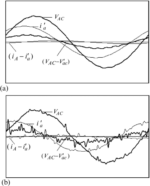
2.8.5 A 15 kVA Three-Phase Transformer Bank Absorbing Power from a PWM Inverter
The same transformer of Section 2.8.4 absorbs power from a PWM inverter [12] (Appendix 3.8) and supplies power to a resistive load (case #1) and to a utility system (case #2). The transformer losses are also measured when supplying a linear resistive load fed from sinusoidal power supply (linear load). All measured data are compared in Table 2.7a.
Table 2.7a
Measured Data of 15 kVA Three-Phase Transformer Connected to PWM Inverter (Fig. 2.57a,b,c)
| Linear load of transformer | Case #1 | Case #2 | |
| vAC | 234.2 Vrms | 234.4 Vrms | 248.2 Vrms |
| 2.93 Arms | 3.30 Arms | 3.82 Arms | |
| 3.56 Vrms | 3.86 Vrms | 4.28 Vrms | |
| 32.4 Arms | 33.3 Arms | 28.2 Arms | |
| Iron-core loss | 232.2 W | 254.6 W | 280.5 W |
| Copper loss | 177.1 W | 172.6 W | 130.4 W |
| Total loss | 409.3 W | 427.2 W | 410.9 W |
| Output power | 13337 W | 13544 W | 12027 W |
| Efficiency | 97.02% | 96.94% | 96.07% |

Measured wave shapes of input voltage, exciting current, series voltage drop, and output current of phase A are shown in Fig. 2.57a,b,c. The total harmonic distortion THDi, K-factor, and harmonic amplitudes of the transformer output current are listed in Table 2.7b.

Table 2.7b
Output Current Harmonics, THDi, and K-Factor (Fig. 2.57b,c)
| Ih(A) | THDi | ||||||
| Case | h = 1 | h = 5 | h = 7 | h = 11 | h = 13 | (%) | K |
| #1 | 32.8 | 0.53 | 0.87 | 0.12 | 0.19 | 5.84 | 1.7 |
| #2 | 28.2 | 1.15 | 1.36 | 0.19 | 0.38 | 10.0 | 2.7 |

Figure 2.58 summarizes the total harmonic distortion (THDi), apparent power (kVA) derating, and real power (kW) derating for uncontrolled (a, b), half-controlled (c), and controlled (d, e) converter loads of transformers. In particular the graphs of Fig. 2.58 can be identified [75] as follows:
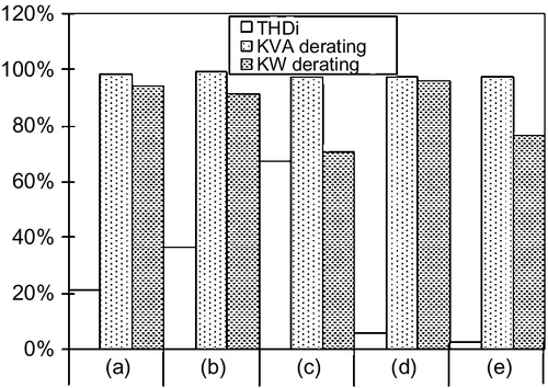
a) 25 kVA single-phase pole transformer [7,11,15,75,76] feeding uncontrolled full wave rectifier load,
b) 4.5 kVA three-phase transformer feeding uncontrolled full wave rectifier load,
c) 4.5 kVA three-phase transformer feeding half-controlled rectifier load,
d) 15 kVA three-phase transformer absorbing power from PWM inverter (14 kW), and
e) 15 kVA three-phase transformer feeding resonant rectifier load (8 kW).
2.8.6 Discussion of Results and Conclusions
2.8.6.1 Discussion of Results
A new approach for the measurement of the derating of three-phase transformers has been described and applied under nonsinusoidal operation. It extends the measurement approach of single-phase transformers [7,73,12,75–77] to three-phase transformers [8,75,76,78].
The apparent power (kVA) derating (Eq. 2-59) of three-phase transformers is not greatly affected by the THDi. Even for THDi values of about 70%, derating is about 99%.
The real power (kW) derating is greatly affected (see Fig. 2.58) by the current wave shape generated by solid-state converters, in particular by the phase shift of the fundamental current component. Therefore, inverters and rectifiers should be designed such that they supply and draw power, respectively, at a displacement (power) factor of about 1.
Three-phase transformers have similar derating properties as single-phase transformers [7,12,73,75–77]. The maximum error of the directly measured losses is about 15%, which compares favorably with the maximum error of more than 60% [7,73] for loss measurement based on the difference between input and output powers as applied to high-efficiency (η > 98%) transformers.
Transformers of the same type may have significantly different iron-core losses as measured in Table 2.3 (100.7 W) and Table 2.5a (65.7 W). Small transformers (kVA range) have relatively small wire cross sections resulting in small skin-effect losses. Large transformers (MW range) have aluminum secondary windings with relatively large wire cross sections resulting in relatively large skin-effect losses. For this reason substation transformers can be expected to have larger apparent power derating than the ones measured in this section. Unfortunately, transformers in the MW range cannot be operated in a laboratory under real-life conditions. Therefore, it is recommended that utilities sponsor the application of the method of this section and permit on-site measurements.
2.8.6.2 Comparison with Existing Techniques
The maximum error of the directly measured losses is about 15% (using potential and current transformers), which compares favorably with the maximum error of more than 60% [7,73] (employing shunts and voltage dividers) for loss measurement based on the difference between input and output powers as applied to high-efficiency (η > 98%) transformers.
The technique of [68] uses the premeasured transformer effective resistance RT as a function of frequency f to calculate transformer total losses for various harmonic currents. This method can be classified as an indirect method because the transformer losses are obtained by computation, instead of direct measurement. In addition, the approach of [68] neglects the fact that the iron-core losses are a function of the harmonic phase shift [69]; in other words, the RT values are not constant for any given harmonic current amplitude but vary as a function of the harmonic voltage amplitude and phase shift as well. Finally, temperature-dependent operating conditions, for example, cannot be considered in [68]. For the above reasons, the method of [68] must be validated by some direct measurements, such as the method presented in this section.
The method of Mocci [70] and Arri et al. [71] has not been practically applied to three-phase transformers. The presented measurement circuit for three-phase transformers [71] uses too many instrument transformers (e.g., nine CTs and nine PTs), and therefore, the measured results will be not as accurate as those based on the measurement circuits of this section, where only four CTs and five PTs are used as shown in Fig. 2.53.
2.9 Summary
This chapter addresses issues related to modeling and operation of transformers under (non)sinusoidal operating conditions. It briefly reviews the operation and modeling of transformers at sinusoidal conditions. It highlights the impact of harmonics and poor power quality on transformer (fundamental and harmonic) losses and discusses several techniques for derating of single- and three-phase transformers including K-factor, FHL-factor, and loss measurement techniques. Several transformer harmonic models in the time domain and/or frequency domain are introduced. Important power quality problems related to transformers such as ferroresonance and geomagnetically induced currents (GICs) are explored. Different techniques for system and transformer grounding are explained. Many application examples explaining nonsinusoidal flux, voltage and current, harmonic (copper and iron-core) loss measurements, derating, ferroresonance, magnetic field strength, propagation of surge, and operation of lightning arresters are presented for further exploration and understanding of the presented materials.
2.10 Problems
Problem 2.1 Pole Transformer Supplying a Residence
Calculate the currents flowing in all branches as indicated in Fig. P2.1 if the pole transformer is loaded as shown. For the pole transformer you may assume ideal transformer relations. Note that such a single-phase configuration is used in the pole transformer (mounted on a pole behind your house) supplying residences within the United States with electricity. What are the real (P), reactive (Q), and apparent (S) powers supplied to the residence?

Problem 2.2 Analysis of an Inductor with Three Coupled Windings
a) Draw the magnetic equivalent circuit of Fig. P2.2.

b) Determine all self- and mutual inductances. Assuming that the winding resistances are known draw the electrical equivalent circuit of Fig. P2.2.
Problem 2.3 Derating of Transformers Based on K-Factor
A substation transformer (S = 10 MVA, VL-L = 5 kV, %PEC-R = 10) supplies a six-pulse rectifier load with the harmonic current spectrum as given by Table X of the paper by Duffey and Stratford [82].
a) Determine the K-factor of the rectifier load.
b) Calculate the derating of the transformer for this nonlinear load.
Problem 2.4 Derating of Transformers Based on FHL-Factor
A substation transformer (S = 10 MVA, VL-L = 5 kV, %PEC-R = 10) supplies a six-pulse rectifier load with the harmonic current spectrum as given by Table X of the paper by Duffey and Stratford [82].
a) Determine the FHL-factor of the rectifier load.
b) Calculate the derating of the transformer for this nonlinear load.
Problem 2.5 Derating of Transformers Based on K-Factor for a Triangular Current Wave Shape
a) Show that the Fourier series representation for the current waveform in Fig. P2.5 is


b) Approximate the wave shape of Fig. P2.5 in a discrete manner, that is, sample the wave shape using 36 points per period and use the program of Appendix 2 to find the Fourier coefficients.
c) Based on the Nyquist criterion, what is the maximum order of harmonic components hmax you can compute in part b? Note that for hmax the approximation error will be a minimum.
d) Calculate the K-factor and the derating of the transformer when supplied with a triangular current wave shape, and %PEC-R = 10. The rated current IR corresponds to the fundamental component of the triangular current.
Problem 2.6 Derating of Transformers Based on K-Factor for a Trapezoidal Current Wave Shape
a) Show that the Fourier series representation for the current waveform in Fig. P2.6 is


b) Approximate the wave shape of Fig. P2.6 in a discrete manner, that is, sample the wave shape using 36 points per period and use the program of Appendix 2 to find the Fourier coefficients.
c) Based on the Nyquist criterion, what is the maximum order of harmonic components hmax you can compute in part b? Note that for hmax the approximation error will be a minimum.
d) Calculate the K-factor and the derating of the transformer when supplied with a trapezoidal current wave shape, and % PEC-R = 10. The rated current IR corresponds to the fundamental component of the trapezoidal current.
Problem 2.7 Force Calculation for a Superconducting Coil for Energy Storage
Design a magnetic storage system which can provide for about 6 minutes a power of 100 MW, that is, an energy of 10 MWh. A coil of radius R = 10 m, height h = 6 m, and N = 3000 turns is shown in Fig. P2.7. The magnetic field strength H inside such a coil is axially directed, essentially uniform, and equal to H = Ni/h. The coil is enclosed by a superconducting box of 2 times its volume. The magnetic field outside the superconducting box can be assumed to be negligible and you may assume a permeability of free space for the calculation of the stored energy.

a) Calculate the magnetic field intensity H and the magnetic flux density B of the coil for constant current i = I0 = 8000 A.
b) Calculate the energy Estored stored in the magnetic field (either in terms of H or B).
c) Determine the radial pressure pradial acting on the coil.
d) Devise an electronic circuit that enables the controlled extraction of the energy from this storage device. You may use bidirectional superconducting switches S1 and S2, which are controlled by a magnetic field via the quenching effect. S1 is ON and S2 is OFF for charging the superconducting coil. S1 is OFF and S2 is ON for the storage time period. S1 is ON and S2 is OFF for discharging the superconducting coil.
Problem 2.8 Measurement of Losses of Delta/Zigzag Transformers
Could the method of Section 2.8 also be applied to a Δ/zigzag three-phase transformer as shown in Fig. P2.8? This configuration is of interest for the design of a reactor [67] where the zero-sequence (e.g., triplen) harmonics are removed or mitigated, and where through phase shifting the 5th and 7th harmonics [83] are canceled.

Problem 2.9 Error Calculations
For a 25 kVA single-phase transformer of Fig. P2.9 with an efficiency of 98.46% at rated operation, the total losses are Ploss = 390 W, where the copper and iron-core losses are Pcu = 325 W and Pfe = 65 W, respectively. Find the maximum measurement errors of the copper Pcu and iron-core Pfe losses as well as that of the total loss Ploss whereby the instrument errors are given in Table P2.9.

Table P2.9
Instruments and Their Error Limits of Fig. P2.9
| Instrument | Full scale | Full-scale errors |
| PT1 | 240 V/240 V | |
| PT2 | 7200 V/240 V | |
| CT1 | 100 A/5 A | |
| CT2 | 5 A/5 A | |
| V1 | 300 V | |
| V2 | 300 V | |
| A1 | 5 A | |
| A2 | 5 A |
Problem 2.10 Delta/Wye Three-Phase Transformer Configuration with Six-Pulse Midpoint Rectifier Employing an Interphase Reactor
a) Perform a PSpice analysis for the circuit of Fig. P2.10, where a three-phase thyristor rectifier with filter (e.g., capacitor Cf) serves a load (Rload). You may assume ideal transformer conditions. For your convenience you may assume (N1/N2) = 1, Rsyst = 0.01 Ω, Xsyst = 0.05 Ω @ f = 60 Hz, ![]() ,
, ![]() , and
, and ![]() . Each of the six thyristors can be modeled by a self-commutated electronic switch and a diode in series, as is illustrated in Fig. E1.1.2 of Application Example 1.1 of Chapter 1. Furthermore, Cf = 500 μF, Lleft = 5 mH, Lright = 5 mH, and Rload = 10 Ω. You may assume that the two inductors Lleft and Lright are not magnetically coupled, that is, Lleftright = 0. Plot one period of either voltage or current after steady state has been reached for firing angles of α = 0°, 60°, and 120°, as requested in parts b to e. Print the input program.
. Each of the six thyristors can be modeled by a self-commutated electronic switch and a diode in series, as is illustrated in Fig. E1.1.2 of Application Example 1.1 of Chapter 1. Furthermore, Cf = 500 μF, Lleft = 5 mH, Lright = 5 mH, and Rload = 10 Ω. You may assume that the two inductors Lleft and Lright are not magnetically coupled, that is, Lleftright = 0. Plot one period of either voltage or current after steady state has been reached for firing angles of α = 0°, 60°, and 120°, as requested in parts b to e. Print the input program.

b) Plot and subject the line-to-line voltages vAB (t), vab(t), and v′ab(t) to Fourier analysis. Why are they different?
c) Plot and subject the input line current iAL (t) of the delta primary to a Fourier analysis. Note that the input line currents of the primary delta do not contain the 3rd, 6th, 9th, 12th,…, that is, harmonic zero-sequence current components.
d) Plot and subject the phase current iAph(t) of the delta primary to a Fourier analysis. Note that the phase currents of the primary delta contain the 3rd, 6th, 9th, 12th,…, that is, harmonic zero-sequence current components.
e) Plot and subject the output voltage vload(t) to a Fourier analysis.
f) How do your results change if the two inductors Lleft and Lright are magnetically coupled, that is, Lleftright = 4.5 mH?
Problem 2.11 Determination of Measurement Uncertainty
Instead of maximum errors, the U.S. Guide to the Expression of Uncertainty in Measurement [84] recommends the use of uncertainty. As an example the uncertainties and the associated correlation coefficients of the simultaneous measurement of resistance and reactance of an inductor having the inductance L and the resistance R are to be calculated. The five measurement sets of Table P2.11 are available for an inductor consisting of the impedance Z = R + jX, where terminal voltage |Ṽt|, current |Ĩt|, and phase-shift angle Φ are measured.
Table P2.11
Measurement Values of the Input Quantities |![]() t|, |Ĩt|, and Φ Obtained from Five Sets of Simultaneous Observations
t|, |Ĩt|, and Φ Obtained from Five Sets of Simultaneous Observations
| Input quantities | |||
| Set number k | Φ (radians) | ||
| 1 | 5.006 | 19.664 | 1.0457 |
| 2 | 4.993 | 19.638 | 1.0439 |
| 3 | 5.004 | 19.641 | 1.0468 |
| 4 | 4.991 | 19.684 | 1.0427 |
| 5 | 4.998 | 19.679 | 1.0433 |

With R = (![]() /
/ ![]() )cosΦ, X = (
)cosΦ, X = (![]() /
/ ![]() )sinΦ, Z = (
)sinΦ, Z = (![]() /
/ ![]() ), and Z2 = R2 + X2 one obtains two independent output quantities – called measurands.
), and Z2 = R2 + X2 one obtains two independent output quantities – called measurands.
a) Calculate the arithmetic means of ![]() ,
, ![]() , and Φ.
, and Φ.
b) Determine the experimental standard deviation of mean of s(![]() ), s(Ī), and s(
), s(Ī), and s(![]() )
)
c) Find the correlation coefficients r(|Ṽt|, |Ĩt|), ![]() and
and ![]() .
.
d) Find the combined standard uncertainty μ ≡ uc(yℓ) of result of measurement where ℓ is the measurand index.
e) Determine the correlation coefficients r(R/X), r(R/Z), and r(X/Z).