
Modeling and Analysis of Induction Machines
Abstract
Investigates the performance of induction machines as a function of the power system’s fundamental and harmonic voltages/currents. It includes sinusoidal model of induction machine, time and space harmonics, forward- and backward-rotating harmonic magnetic fields, and magnetic field- and torque calculations based on the finite-difference method. The steady-state stability of rotating machines is reviewed, and the extension of the variable-speed range is obtained through compensation of flux weakening. Fundamental, integer, inter-, fractional and sub-harmonic torque characteristics of three-phase induction machines are analysed. The interaction of space and time harmonics, voltage-stress winding failures, classification and available harmonic models of induction machines as well as discussions of rotor eccentricity are provided. 14 application examples with solutions and 14 application-oriented problems are listed.
Before the development of the polyphase AC concept by Nikola Tesla [1] in 1888, there was a competition between AC and DC systems. The invention of the induction machine in the late 1880s completed the AC system of electrical power generation, transmission, and utilization. The Niagara Falls hydroplant was the first large-scale application of Tesla’s polyphase AC system. The theory of single- and three-phase induction machines was developed during the first half of the twentieth century by Steinmetz [2], Richter [3], Kron [4], Veinott [5], Schuisky [6], Bödefeld [7], Alger [8], Fitzgerald et al. [9], Lyon [10], and Say [11] – just to name a few of the hundreds of engineers and scientists who have published in this area of expertise. Newer textbooks and contributions are by Match [12], Chapman [13], and Fuchs et al. [14,15]. In these works mostly balanced steady-state and transient performances of induction machines are analyzed. Most power quality problems as listed below are neglected in these early publications because power quality was not an urgent issue during the last century.
Today, most industrial motors of one horsepower or larger are three-phase induction machines. This is due to their inherent advantages as compared with synchronous motors. Although synchronous motors have certain advantages – such as constant speed, generation of reactive power (leading power factor based on consumer notation of current) with an overexcited field, and low cost for low-speed motors – they have the constraints of requiring a DC exciter, inflexible speed control, and high cost for high-speed motors. The polyphase induction motors, however, have certain inherent advantages, including these:
• Induction motors require no exciter (no electrical connection to the rotor windings except for some doubly excited machines);
• They are rugged and relatively inexpensive;
• They require very little maintenance;
• They have nearly constant speed (slip of only a few percent from no load to full load);
• They are suitable for explosive environments;
• Starting of motors is relatively easy; and
• Operation of three-phase machines within a single-phase system is possible.
The main disadvantages of induction motors are:
• high starting current if no starters are relied on, and
• low and lagging (based on consumer notation of current) power factor at light loads.
For most applications, however, the advantages far outweigh the disadvantages. In today’s power systems with a large number of nonlinear components and loads, three-phase induction machines are usually subjected to nonsinusoidal operating conditions. Conventional steady-state and transient analyses do not consider the impact of voltage and/or current harmonics on three-phase induction machines. Poor power quality has many detrimental effects on induction machines due to their abnormal operation, including:
• excessive voltage and current harmonics,
• excessive saturation of iron cores,
• static and dynamic rotor eccentricities,
• one-sided magnetic pull due to DC currents,
• shaft fluxes and associated bearing currents,
• mechanical vibrations,
• dynamic instability when connected to weak systems,
• premature aging of insulation material caused by cyclic operating modes as experienced by induction machines for example in hydro- and wind-power plants,
• increasing core (hysteresis and eddy-current) losses and possible machine failure due to unacceptably high losses causing excessive hot spots,
• increasing (fundamental and harmonic) copper losses,
• reduction of overall efficiency,
• generation of inter- and subharmonic torques,
• production of (harmonic) resonance and ferroresonance conditions,
• failure of insulation due to high voltage stress caused by rapid changes in supply current and lightning surges,
• unbalanced operation due to an imbalance of power systems voltage caused by harmonics, and
• excessive neutral current for grounded machines.
These detrimental effects call for the understanding of the impact of harmonics on induction machines and how to protect them against poor power quality conditions. A harmonic model of induction motors is essential for loss calculations, harmonic torque calculations, derating analysis, filter design, and harmonic power flow studies.
This chapter investigates the behavior of induction machines as a function of the harmonics of the power system’s voltages/currents, and introduces induction machine harmonic concepts suitable for loss calculations and harmonic power flow analysis. After a brief review of the conventional (sinusoidal) model of the induction machine, time and space harmonics as well as forward- and backward-rotating magnetic fields at harmonic frequencies are analyzed. Some measurement results of voltage, current, and flux density waveforms and their harmonic components are provided. Various types of torques generated in induction machines, including fundamental and harmonic torques as well as inter- and subharmonic torques, are introduced and analyzed. The interaction of space and time harmonics is addressed. A section is dedicated to voltage-stress winding failures of AC machines fed by voltage-source and current-source pulse-width-modulated (PWM) inverters. Some available harmonic models of induction machines are briefly introduced. The remainder of the chapter includes discussions regarding rotor eccentricity, classification of three-phase induction machines, and their operation within a single-phase system. This chapter contains a number of application examples to further clarify the relatively complicated issues.
3.1 Complete sinusoidal equivalent circuit of a three-phase induction machine
Simulation of induction machines under sinusoidal operating conditions is a well-researched subject and many transient and steady-state models are available. The stator and rotor cores of an induction machine are made of ferromagnetic materials with nonlinear (B–H) or (λ – i) characteristics. As mentioned in Chapter 2, magnetic coils exhibit three types of nonlinearities that complicate their analysis: saturation effects, hysteresis loops, and eddy currents. These phenomena result in nonsinusoidal flux, voltage and current waveforms in the stator and rotor windings, and additional copper (due to current harmonics) and core (due to hysteresis loops and eddy currents) losses at fundamental and harmonic frequencies. Under nonsinusoidal operating conditions, the stator magnetic field will generate harmonic rotating fields that will produce forward- and backward-rotating magnetomotive forces (mmfs); in addition to the time harmonics (produced by the nonsinusoidal stator voltages), space harmonics must be included in the analyses. Another detrimental effect of harmonic voltages at the input terminals of induction machines is the generation of unwanted harmonic torques that are superimposed with the useful fundamental torque, producing vibrations causing a deterioration of the insulation material and rotor copper/aluminum bars. Linear approaches for induction machine modeling neglect these nonlinearities (by assuming linear (λ – i) characteristics and sinusoidal current and voltage waveforms) and use constant values for the magnetizing inductance and the core-loss resistance.
Sinusoidal modeling of induction machines is not the main subject of this chapter. However, Fig. 3.1 illustrates a relatively simple and accurate frequency-based linear model that will be extended to a harmonic model in Sections 3.4 to 3.9. In this figure subscript 1 denotes the fundamental frequency (h = 1); ω1 and s1 are the fundamental angular frequency (or velocity) and the fundamental slip of the rotor, respectively. Rfe is the core-loss resistance, Lm is the (linear) magnetizing inductance, Rs, R′r, Lsℓ, and L′rℓ are the stator and the rotor (reflected to the stator) resistances and leakage inductances, respectively [3–15]. The value of Rfe is usually very large and can be neglected. Thus, the simplified sinusoidal equivalent circuit of an induction machine results, as shown in Fig. 3.2.


Replacing the network to the left of line a–b by Thevenin’s theorem (TH) one gets


Using Eq.3-1, the Thevenin adjusted equivalent circuit is shown in Fig. 3.3.

The fundamental (h = 1) slip is
where ns1 is the synchronous speed of the stator field, nm is the (mechanical) speed of the rotor, and ωs1, ωm are the corresponding angular velocities (or frequencies), respectively. Note that subscript 1 denotes fundamental frequency.
For a p-pole machine,

where ω1 = 2π f1 = 377 rad/s is the fundamental angular velocity (frequency).
The torque of a three-phase (q1 = 3) induction machine is (if ![]() )
)

or

or

or

For small values of s1 we have

This relation is called the small-slip approximation for the torque.
Based on Eq. 3-4, the fundamental torque-speed characteristic of a three-phase induction machine is shown in Fig. 3.4.

Mechanical output power (neglecting iron-core losses, friction, and windage losses) is
The air-gap power is (Fig. 3.5)

where ![]()

The loss distribution within the machine is given in Fig. 3.6. Note that
and

The complete fundamental torque-speed relation detailing braking, motoring, and generation regions is shown in Fig. 3.7, where ns1 denotes the synchronous (mechanical) speed of the fundamental rotating magnetic field.

3.1.1 Application Example 3.1: Steady-State Operation of Induction Motor at Undervoltage
A Pout = 100 hp, VL-L_rat = 480 V, f = 60 Hz, p = 6 pole, three-phase induction motor runs at full load and rated voltage with a slip of 3%. Under conditions of stress on the power system, the line-to-line voltage drops to VL-L_low = 430 V. If the load is of the constant torque type, compute for the lower voltage:
a) Slip slow (use small-slip approximation).
b) Shaft speed nm_low in rpm.
c) Output power Pout_low.
d) Rotor copper loss Pcur_low = (Ir′)2Rr′ in terms of the rated rotor copper loss at rated voltage.
Solution to Application Example 3.1
a) Based on the small-slip approximation ![]() , the new slip at the low voltage is
, the new slip at the low voltage is
b) With the synchronous speed ![]() one calculates the shaft speed at low voltage as
one calculates the shaft speed at low voltage as
c) The output power at low voltage is Pout = ωm · Tm. For constant mechanical torque one gets ![]()
d) Due to the relation ![]() (where Pg is the air-gap power), the torque is proportional to Pg, and therefore, for constant torque operation the air-gap power is constant. Thus the rotor loss is
(where Pg is the air-gap power), the torque is proportional to Pg, and therefore, for constant torque operation the air-gap power is constant. Thus the rotor loss is ![]()
One concludes that a decrease of the terminal voltage increases the rotor loss (temperature) of an induction motor.
3.1.2 Application Example 3.2: Steady-State Operation of Induction Motor at Overvoltage
Repeat Application Example 3.1 for the condition when the line-to-line voltage of the power supply system increases to VL-L_high = 510 V.
Solution to Application Example 3.2
a) Based on the small-slip approximation ![]() the new slip at the high voltage is
the new slip at the high voltage is
b) With the synchronous speed ![]() one calculates the shaft speed at high voltage as nm_high = (1 – shigh)n = (1 – 0.02657)(1200) = 1168.11 rpm.
one calculates the shaft speed at high voltage as nm_high = (1 – shigh)n = (1 – 0.02657)(1200) = 1168.11 rpm.
c) The output power at high voltage is Pout = ωm · Tm. For constant mechanical torque one gets ![]()
d) Due to the relation ![]() , where Pg is the air-gap power, the torque is proportional to Pg, and therefore, for constant torque operation the air-gap power is constant. Thus the rotor loss is Pcur_high = shighPg =
, where Pg is the air-gap power, the torque is proportional to Pg, and therefore, for constant torque operation the air-gap power is constant. Thus the rotor loss is Pcur_high = shighPg = ![]() Pcur_rat = 0.886 Pcur_rat.
Pcur_rat = 0.886 Pcur_rat.
One concludes that an increase of the terminal voltage decreases the rotor loss (temperature) of an induction motor.
3.1.3 Application Example 3.3: Steady-State Operation of Induction Motor at Undervoltage and Under-Frequency
Repeat Application Example 3.1 for the condition when the line-to-line voltage of the power supply system and the frequency drop to VL-L_low = 430 V and flow = 59 Hz, respectively.
Solution to Application Example 3.3
The small-slip approximation results in the torque equation ![]()
a) Applying the relation to rated conditions (1) one gets ![]()
Applying the relation to low-voltage and low-frequency conditions (2) one gets ![]()
With T(1) = T(2) and the relations ![]()
one obtains ![]()
b) The synchronous speed ns(2) at f(2) = 59 Hz is ![]() , or the corresponding shaft speed
, or the corresponding shaft speed ![]()
c) The torque-output power relations are 
With T(1) = T(2) one gets  or
or ![]() or
or  For the reduced output power it follows
 ![]()
d) The copper losses of the rotor are ![]() and the output power is
and the output power is ![]() The application of the relations to the two conditions (1) and (2) yields
The application of the relations to the two conditions (1) and (2) yields

The rotor loss increase becomes now ![]()
One concludes that the simultaneous reduction of voltage and frequency increases the rotor losses (temperature) in a similar manner as discussed in Application Example 3.1. It is advisable not to lower the power system voltage beyond the levels as specified in standards.
3.2 Magnetic fields of three-phase machines for the calculation of inductive machine parameters
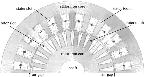
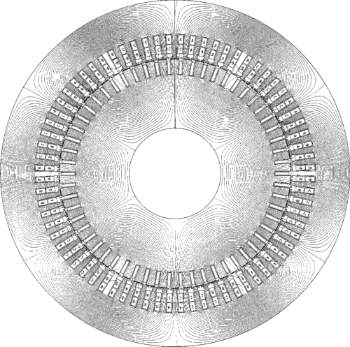
Numerical approaches such as the finite-difference and finite-element methods [16] enable engineers to compute no-load and full-load magnetic fields and those associated with short-circuit and starting conditions, as well as fields for the calculation of stator and rotor inductances/reactances. Figures 3.8 and 3.9 represent the no-load fields of four- and six-pole induction machines [17,18]. Figure 3.10a–e illustrates radial forces generated as a function of the rotor position. Such forces cause audible noise and vibrations. The calculation of radial and tangential magnetic forces is discussed in Chapter 4 (Section 4.2.14), where the concept of the “Maxwell stress” is employed. Figures 3.11 to 3.13 represent unsaturated stator and rotor leakage fields and the associated field during starting of a two-pole induction motor. Figures 3.14 and 3.15 represent saturated stator and rotor leakage fields, respectively, and Fig. 3.16 depicts the associated field during starting of a two-pole induction machine. The starting current and starting torque as a function of the terminal voltage are shown in Fig. 3.17 [19]. This plot illustrates how saturation influences the starting of an induction motor. Note that the linear (hand) calculation results in lower starting current and torque than the numerical solution.


Any rotating machine design is based on iterations. No closed form solution exists because of the nonlinearities (e.g., iron-core saturation) involved. In Fig. 3.13 the field for the first approximation, where saturation is neglected and a linear B–H characteristic is assumed, permits us to calculate stator and rotor currents for which the starting field can be computed under saturated conditions assuming a nonlinear (B–H) characteristic as depicted in Fig. 3.16. For the reluctivity distribution caused by the saturated short-circuit field the stator (Fig. 3.14) and rotor (Fig. 3.15) leakage reactances can be recomputed, leading to the second approximation as indicated in Fig. 3.16. In practice a few iterations are sufficient to achieve a satisfactory solution for the starting torque as a function of the applied voltage as illustrated in Fig. 3.17. It is well known that during starting saturation occurs only in the stator and rotor teeth and this is the reason why Figs. 3.13 and 3.16 are similar.
3.3 Steady-state stability of a three-phase induction machine
The steady-state stability criterion is [20]

where TL is the load torque and T is the motor torque. Using this equation, the stable steady-state operating point of a machine for any given load-torque characteristic can be determined.
3.3.1 Application Example 3.4: Unstable and Stable Steady-State Operation of Induction Machines
Figure E3.4.1 shows the torque–angular velocity characteristic of an induction motor (T – ωm) supplying a mechanical constant torque load (TL). Determine the stability of the operating points Q1 and Q2.

Solution to Application Example 3.4
The stability conditions at the two points where the two curves intersect are


Therefore, operation at Q1 is unstable and will result in rapid speed reduction. This will stop the operation of the induction machine, while operating point Q2 is stable.
3.3.2 Application Example 3.5: Stable Steady-State Operation of Induction Machines
Figure E3.5.1 shows the torque–angular velocity relation (T – ωm) of an induction motor supplying a mechanical load with nonlinear (parabolic) torque (TL). Determine the stability of the operating point Q1.

Solution to Application Example 3.5
The stability conditions at the point where the two curves intersect is

Therefore, an induction machine connected to a mechanical load with parabolic torque-speed characteristics as shown in Fig. E3.5.1 will not experience any steady-state stability problems.
3.3.3 Resolving Mismatch of Wind-Turbine and Variable-Speed Generator Torque–Speed Characteristics
It is well known that the torque–speed characteristic of wind turbines (Fig. 3.18) and commonly available variable-speed drives employing field weakening (Fig. 3.19a) do not match because the torque of a wind turbine is proportional to the square of the speed and that of a variable-speed drive is inversely proportional to the speed in the field-weakening region. One possibility to mitigate this mismatch is an electronic change in the number of poles p or a change of the number of series turns of the stator winding [21–23]. The change of the number of poles is governed by the relation

where Bmax is the maximum flux density at the radius R of the machine, Nrat is the rated number of series turns of a stator phase winding, and L is the axial iron-core length of the machine.

 nm2.
nm2.
 1/nm in field-weakening region. The full line corresponds to the torque T and the dashed-dotted line to the power P. (b) Variable-speed drive torque–speed characteristic by changing the number of series turns of the stator winding from Nrat to Nrat/2. The full line corresponds to the torque T and the dashed-dotted line to the power P. (c) Measured variable-speed drive response with winding switching from pole number p1 to p2 resulting in a speed range from 600 to 4000 rpm [21]. One horizontal division corresponds to 200 ms. One vertical division corresponds to 800 rpm.
The change of the number of turns N is governed by

The introduction of an additional degree of freedom – either by a change of p or N – permits an extension of the constant flux region. Adding this degree of freedom will permit wind turbines to operate under stalled conditions at all speeds, generating maximum power at a given speed with no danger of a runaway. This will make the blade-pitch control obsolete – however, a furling of the blades at excessive wind velocities must be provided – and wind turbines become more reliable and less expensive due to the absence of mechanical control. Figure 3.19b illustrates the speed and torque increase due to the change of the number of turns from Nrat to Nrat/2, and Fig. 3.19c demonstrates the excellent dynamic performance of winding switching with solid-state switches from number of poles p1 to p2 [21]. The winding reconfiguration occurs near the horizontal axis (small slip) at 2400 rpm.
3.4 Spatial (space) harmonics of a three-phase induction machine
Due to imperfect (e.g., nonsinusoidal) winding distributions and due to slots and teeth in stator and rotor, the magnetomotive forces (mmfs) of an induction machine are nonsinusoidal.
For sinusoidal distribution one obtains the mmfs

Note that cos(θ – 240°) = cos(θ + 120°). For nonsinusoidal mmfs (consisting of fundamental, third, and fifth harmonics) one obtains

where

The magnetomotive force (mmf) originates in the phase belts a–a’, b–b’, and c–c’ as shown in Fig. 3.20.

The total mmf is
where
Note that cos x cos y = ½{cos(x – y) + cos(x + y)}; therefore,

Correspondingly,


Therefore, with Eq. 3-12 the total mmf is simplified:
The angular velocity of the fundamental mmf ![]() is
is

and the angular velocity of the 5th space harmonic mmf ![]() is
is

Graphical representation of spatial harmonics (in the presence of fundamental, third, and fifth harmonics mmfs) with phasors is shown in Fig. 3.21. Note that the 3rd harmonic mmf cancels (is equal to zero).

Similar analysis is performed to determine the rotating directions of each individual space harmonic, and the positive-, negative-, and zero-sequence harmonic orders can be defined, as listed in Table 3.1.
Table 3.1
Positive-, Negative-, and Zero-Sequence Spatial Harmonics
| Spatial-harmonic sequence | + | – | 0 |
| Spatial-harmonic order | 1 | 2 | 3 |
| 4 | 5 | 6 | |
| 7 | 8 | 9 | |
| 10 | 11 | 12 | |
| 13 | 14 | 15 | |
| . | . | . |

Note that:
Even and triplen harmonics are normally not present in a balanced three-phase system!
In general one can write for spatial harmonics

where +, –, and 0 are used for positive-, negative-, and zero-sequence space harmonic orders, respectively. Figure 3.22 illustrates the superposition of fundamental mmf with 5th space harmonic resulting in amplitude modulation where fundamental of 60 Hz is modulated with 12 Hz.

3.5 Time harmonics of a three-phase induction machine
A three-phase induction machine is excited by balanced three-phase f1 = 60 Hz currents containing a fifth time harmonic. The equations of the currents are for ω1 = 2πf1:

Note that the three-phase system rotates in a clockwise (cw) manner; that is, in a mathematically negative sense. Assume that the winding has been designed to eliminate all spatial harmonics. Thus for phase a the mmf becomes
Correspondingly,

The total mmf is
expanded:

or

The angular velocity of the fundamental ![]() is
is
and the angular velocity of the fifth time harmonic ![]() is
is
For the current system (consisting of the fundamental and 5th harmonic components where the 5th harmonic system rotates in counterclockwise direction)

the fifth time harmonic has the angular velocity

Phasor representation for forward rotating fundamental and forward rotating 5th harmonic current systems is given in Fig. 3.23. Phasor representation for forward rotating fundamental and backward rotating 5th harmonic current systems is shown in Fig. 3.24.


Similar analysis can be performed to determine the rotating directions of each individual time harmonic and to define the positive-, negative-, and zero-sequence harmonic orders, as listed in Table 3.2. As with the space harmonics, even and triplen harmonics are normally not present, provided the system is balanced.
Table 3.2
Positive-, Negative-, and Zero-Sequence Time Harmonics
| Time-harmonic sequence | + | – | 0 |
| Time-harmonic order | 1 | 2 | 3 |
| 4 | 5 | 6 | |
| 7 | 8 | 9 | |
| 10 | 11 | 12 | |
| 13 | 14 | 15 | |

In general one can write for time harmonics

where +, –, and 0 are used for positive-, negative-, and zero-sequence time harmonic orders, respectively.
Therefore, time harmonics voltages have an important impact on induction machines. Forward- and backward-rotating fields are produced by positive-, negative-, and zero-sequence harmonics that produce harmonic shaft torques.
3.6 Fundamental and harmonic torques of an induction machine
Starting with the Thevenin-adjusted circuit as illustrated in Fig. 3.25, one obtains the current of the hth harmonic


Therefore, the electrical torque for the hth harmonic is

Similarly, the fundamental (h = 1) torque is
3.6.1 The Fundamental Slip of an Induction Machine
The fundamental slip is
or
where ![]() is the (mechanical) synchronous fundamental angular velocity and ωm is the mechanical angular shaft velocity.
is the (mechanical) synchronous fundamental angular velocity and ωm is the mechanical angular shaft velocity.
The fundamental torque referred to fundamental slip s1 is shown in Fig. 3.26 where Te1 is the machine torque and TL is the load torque. If Rs = 0 then Te1 is symmetric to the point at (Te1 = 0/s1 = 0) or (Te1 = 0/ωs1).

3.6.2 The Harmonic Slip of an Induction Machine
The harmonic slip (without addressing the direction of rotation of the harmonic field) is defined as

where ωs1 = (ω1)/(p/2) and ω1 is the electrical angular velocity, ω1 = 2πf1 and f1 = 60 Hz.
To include the direction of rotation of harmonic mmfs, in the following we assume that the fundamental rotates in forward direction, the 5th in backward direction, and the 7th in forward direction (see Table 3.2 for positive-, negative-, and zero-sequence components).
For motor operation ωm < ωs1; thus for the 5th harmonic component, one obtains

where (–5ωs1) means rotation in backward direction, or

Note that in this equation 5ωs1 is the base (reference) angular velocity.
Correspondingly, one obtains for the forward rotating 7th harmonic:

where 7ωs1 is the base.
Therefore, the harmonic slip is

Harmonic torques Te7 and Te5 (as a function of the angular velocity ωm and the harmonic slips s7 and s5) are depicted in Figs. 3.27 and 3.28, respectively.


3.6.3 The Reflected Harmonic Slip of an Induction Machine
If ωs1 is taken as the reference angular velocity, then for the backward rotating fifth harmonic one obtains

where s5(1) is the reflected fifth harmonic slip.
Correspondingly, if one takes ωs1 as reference then for the forward rotating seventh harmonic one gets

where s7(1) is the reflected seventh harmonic slip.
In general, the reflected harmonic slip is

To understand the combined effects of fundamental and harmonic torques, it is more convenient to plot harmonic torques (Teh) as a function of the reflected harmonic slips (sh(1)):
• The harmonic torque Te7 reflected to harmonic slip ![]() is depicted in Fig. 3.29; and
is depicted in Fig. 3.29; and

• The harmonic torque Te5 reflected to harmonic slip ![]() is shown in Fig. 3.30.
is shown in Fig. 3.30.

3.6.4 Reflected Harmonic Slip of an Induction Machine in Terms of Fundamental Slip
The relation between s1 (fundamental slip) and sh(1) (reflected harmonic slip) is

Therefore, the reflected harmonic slip, in terms of fundamental slip, is
For the backward rotating 5th harmonic one gets
and for the forward rotating 7th harmonic
Note that
In general, the reflected harmonic slip sh(1) for the forward and the backward rotating harmonics is a linear function of the fundamental slip s1:

Superposition of fundamental (h = 1), fifth harmonic (h = 5), and seventh harmonic (h = 7) torque Te = Te1 + Te5 + Te7 is illustrated in Fig. 3.31. At ωm = ωmrated the total electrical torque Te is identical to the load torque TL or Te1 + Te5 + Te7 = TL, where Te1 is a motoring torque, Te7 is a motoring torque, and Te5 is a braking torque. Figure 3.32 shows the graphical phasor representation of superposition of torques as given in Fig. 3.31.


3.6.5 Reflected Harmonic Slip of an Induction Machine in Terms of Harmonic Slip
In this section, the relation between the reflected harmonic slip sh(1) and the harmonic slip sh is determined as ![]()
The harmonic slip (without addressing the direction of rotation of the harmonic field) is

with
It follows that

With ![]() , one obtains for forward rotating harmonics
, one obtains for forward rotating harmonics
or

Similar analysis can be used for backward-rotating harmonics. Therefore, sh(1) is a linear function of sh:
3.7 Measurement results for three- and single-phase induction machines
Measurement techniques for the determination of the (copper and iron-core) losses of induction machines are described in [24]. The losses of harmonics of single-phase induction motors are measured in [25]. Typical input current wave shapes for single-and three-phase induction motors fed by thyristor converters are depicted in Figs. 3.33 and 3.34 [26]. In addition to semiconductor converters, harmonics can be generated by the DC magnetization of transformers [27]. A summary of the heating effects due to harmonics on induction machines is given in [28]. The generation of sub- and interharmonic torques by induction machines is presented in [29]. Power quality of machines relates to harmonics of the currents and voltages as well as to those of flux densities. The latter are more difficult to measure because sensors (e.g., search coils, Hall devices) must be implanted in the core. Nevertheless, flux density harmonics are important from an acoustic noise [30] and vibration [31–33] point of view. Excessive vibrations may lead to a reduction of lifetime of the machine. Single-phase induction machines are one of the more complicated electrical apparatus due to the existence of forward- and backward-rotating fields. The methods as applied to these machines are valid for three-phase machines as well, where only forward fundamental rotating fields exist.


3.7.1 Measurement of Nonlinear Circuit Parameters of Single-Phase Induction Motors
The optimization of single- and three-phase induction machines is based on sinusoidal quantities neglecting the influence of spatial and time harmonics in flux densities, voltages, and currents [14,15,34,35]. At nonsinusoidal terminal voltages, the harmonic losses of single-phase induction motors impact their efficiency [25]. The computer-aided testing of [24] will be relied on to measure nonlinear circuit parameters and flux densities in stator teeth and yokes as well as in the air gap of permanent-split-capacitor (PSC) motors. Detailed test results are presented in [36]. One concludes that tooth flux density wave shapes can be nearly sinusoidal although the exciting or magnetizing currents are nonsinusoidal.
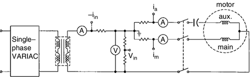
A computer-aided testing (CAT) circuit and the computer-aided testing of electrical apparatus program (CATEA) are used in [24] to measure nonlinear parameters. The CAT circuit is shown in Fig. 3.35, where four-channel signals vm, im, va, and ia corresponding to main (m) and auxiliary (a) phase voltages and currents, respectively, are sampled by a personal computer via a 12-bit A/D converter.

Three (see Table 3.3) fractional horsepower PSC single-phase induction motors serving as prime movers for window air conditioners are tested and their parameters listed.
Table 3.3
Three Fractional Horsepower PSC Single-Phase Induction Motors Serving as Prime Movers for Window Air Conditioners
| Single-phase motor R333MC | Capacitor: 15 μF, 370 V, output power: 1/2 hp |
| Single-phase motor Y673MG1 | Capacitor: 17.5 μF, 366 V, output power: 3/4 hp |
| Single-phase motor 80664346 | Capacitor: 25 μF, 370 V, output power: 1/2 hp |
All motors to be tested are operated at minimum load, where input and output lines at the compressor are open to air. Measurements are conducted at an ambient temperature of 22°C. The linear stator leakage impedance of a motor is measured by removing the rotor from the stator bore and applying various terminal voltage amplitudes to the stator windings. When the main-phase parameters are measured, the switch leading to the auxiliary phase must be open, and vice versa. From the sampled data one obtains the fundamental voltages and currents of the main- and auxiliary-phase windings through Fourier analysis.
Stator Impedance
The stator input resistance and reactance are derived via linear regression. The stator leakage reactance is obtained by subtracting the reactance corresponding to leakage flux inside the bore of the motor from its input reactance [25].
Rotor Impedance
The rotor leakage impedance is frequency dependent and nonlinear because of the closed-rotor slots. The rotor impedance, referred to the main-phase winding, is measured by passing varying amplitudes of current – from about 5 to 150% of rated current – through the main-phase winding under locked-rotor conditions. The total input resistance is derived from linear regression and the rotor resistance at rated frequency is obtained by subtracting the main-phase stator winding resistance from the total input resistance. The rotor resistance, taking the skin effect into account, can be obtained from [25]:

where
In Eq. 3-34b, f is the frequency of the rotor current. kr is the skin-effect coefficient derived from the height of the rotor slot hr and the resistivity of the bar ρr:

In Eq. 3-33, Rr0 is the DC rotor resistance that can be derived from the rotor AC resistance at rated frequency and its skin-effect coefficient. The nonlinear rotor leakage reactance as a function of the amplitude of the rotor current – which can be described by a (λ – i) characteristic – is obtained by subtracting the stator main-phase winding leakage reactance from the total input reactance. A linear rotor leakage reactance – which can be used as an approximation of the nonlinear rotor leakage reactance – is also derived from a linear regression.
Magnetizing Impedance
The magnetizing (λ – i) characteristic referred to the stator main-phase winding is measured by supplying varying amplitudes of voltage to the main-phase winding at no-load operation. The forward induced voltage is determined by subtracting from the input voltage the voltage drop across the stator impedance and the backward induced voltage (the voltage drop across the rotor backward equivalent impedance); note that in [25, Fig. 7a], the main-phase forward circuit, and [25, Fig. 7c], the main-phase backward circuit, are connected in series, whereby h = 1. Thereafter, the magnetizing impedance is derived from the ratio of the forward induced voltage and the input current in the frequency (fundamental) domain. The magnetizing reactance as a function of the amplitude of the forward induced voltage is derived from the imaginary part of the (complex) magnetizing impedance.
The (λ – i) characteristics are given in the frequency domain, which means that both λ (flux linkages) and i (current) have fundamental amplitudes only. The fundamental amplitudes of either flux linkages or currents can be derived from each other via such characteristics.
Iron-Core Resistance
The resistance corresponding to the iron-core loss is determined as follows. The iron-core and the mechanical frictional losses are computed by subtracting from the input power at no load
1. the copper loss of the main-phase winding at no load,
2. the backward rotor loss at no load, and
3. the forward air-gap power responsible for balancing the backward rotor loss.
Thereafter, the iron-core and the mechanical frictional losses, the total value of which is a linear function of the square of the forward induced voltage, are separated by linear regression. The equivalent resistance corresponding to the iron-core loss is derived from the slope of the regression line.
Turns Ratio between the Turns of the Main- and Auxiliary-Phase Windings
The ratio between the turns of the main- and auxiliary-phase windings ![]() is also an important parameter for single-phase induction motors. The main- and auxiliary-phase windings of some motors are not placed in spatial quadrature; therefore, an additional parameter θ, the spatial angle between the axes of the two stator windings, must be determined. These two parameters
is also an important parameter for single-phase induction motors. The main- and auxiliary-phase windings of some motors are not placed in spatial quadrature; therefore, an additional parameter θ, the spatial angle between the axes of the two stator windings, must be determined. These two parameters ![]() are found by measuring the main-phase induced voltage and current as well as the auxiliary-phase induced voltage when the motor is operated at no load. As has been mentioned above, the main-phase forward (f) and backward (b) induced voltages in the frequency domain, Ẽf and Ẽb, respectively, can be obtained from the input voltage and current. If
are found by measuring the main-phase induced voltage and current as well as the auxiliary-phase induced voltage when the motor is operated at no load. As has been mentioned above, the main-phase forward (f) and backward (b) induced voltages in the frequency domain, Ẽf and Ẽb, respectively, can be obtained from the input voltage and current. If
is used to represent this complex turns ratio, then the auxiliary-phase induced voltage is given by
Therefore, the complex ratio ![]() can be iteratively computed from
can be iteratively computed from
where ![]() is the complex conjugate of
is the complex conjugate of ![]() . Measured parameters of PSC motors are given in Section 3.7.2.
. Measured parameters of PSC motors are given in Section 3.7.2.
3.7.1.1 Measurement of Current and Voltage Harmonics
Voltage and current harmonics can be measured with state-of-the-art equipment [24–26]. Voltage and current waveshapes representing input and output voltages or currents of thyristor or triac controllers for induction motors are presented in Figs. 3.33 and 3.34. Here it is important that DC currents due to the asymmetric gating of the switches do not exceed a few percent of the rated controller current; DC currents injected into induction motors cause braking torques and generate additional losses or heating [26,28,41].
3.7.1.2 Measurement of Flux-Density Harmonics in Stator Teeth and Yoke (Back Iron)
Flux densities in the teeth of rotating machines are of the alternating type, whereas those in the yoke (back iron) are of the rotating type. The loss characteristics for both types are different and these can be requested from the electrical steel manufacturers. The motors to be tested are mounted on a testing frame, and measurements are performed under no load or minimum load with rated run capacitors. Four stator search coils with N = 3 turns each are employed to indirectly sense the flux densities of the teeth and yoke located in the axes of the main- and auxiliary-phase windings (see Fig. 3.36). The induced voltages in the four search coils are measured with two different methods: the computer sampling and the oscilloscope methods.

Measurement via Computer Sampling
The computer-aided testing circuit and program [24] are relied on to measure the induced voltages of the four search coils of Fig. 3.36. The CAT circuit is shown in Figs. 3.36 and 3.37, where eight channel signals (vin, iin, im, ia, emt, eat, emy, and eay corresponding to input voltage and current, main- and auxiliary-phase currents, main- and auxiliary-phase tooth search-coil induced voltages, and main- and auxiliary-phase yoke (back iron)-search coil induced voltages, respectively), are sampled [36].
The flux linkages of the search coils are defined as

and numerically obtained from
The average or DC value is

or the AC values are
where e(t) of Eq. 3-38 is the induced voltage measured in a search coil and n in Eqs. 3-39 to 3-41 is the number of sampled points. The maximum flux linkage λmax can be obtained from λi. The maximum flux density is given by
where the number of turns of each search coil is N = 3 and s is given for a stator tooth and yoke by the following equations:
where wt, hy, l, and kfe are the width of the (parallel) stator teeth (where two search coils reside), the height of the yoke or stator back iron (where two search coils reside), the length of the iron core, and the iron-core stacking factor, respectively. Measured data of PSC motors at rated voltage are presented in Section 3.7.2.
The maximum flux densities in stator teeth and yoke at the axes of the main- and auxiliary-phase windings are measured for various voltage amplitudes by recording the induced voltages in the four search coils. A digital oscilloscope is used to plot the induced voltages of the search coils. These waveforms are then sampled either by hand or by computer based on 83 points per period. Complex Fourier series components ![]() are computed – taking into account the Nyquist criterion – and the integration is performed in the complex domain as follows:
are computed – taking into account the Nyquist criterion – and the integration is performed in the complex domain as follows:


The maximum flux linkage λmax is found from λ(t) and the maximum flux densities are determined from Eqs. 3-42 to 3-44.
3.7.2 Application Example 3.6: Measurement of Harmonics within Yoke (Back Iron) and Tooth Flux Densities of Single-Phase Induction Machines
The three permanent-split capacitor (PSC) motors (R333MC, Y673MG1, and 80664346) of Table 3.3 are subjected to the tests described in the prior subsections of Section 3.7, and pertinent results will be presented. These include stator, rotor, and magnetizing parameters, and tables listing no-load input impedances of the main and auxiliary phases (Tables E3.6.1 and E3.6.2). The bold data of the tables correspond to rated main- and auxiliary-phase voltages at no load. The rated auxiliary-phase voltage is obtained by multiplying the rated main-phase voltage with the measured turns ratio ![]() . Lm and La are inductances of the main- and auxiliary-phase windings, respectively.
. Lm and La are inductances of the main- and auxiliary-phase windings, respectively.
Table E3.6.1
Main-Phase (m) Input Impedance at Single-Phase No-Load Operation as a Function of Input Voltage for R333MC
| Vm (V) | Rm (Ω) | Xm (Ω) | Zm (Ω) | Lm (mH) |
| 250.3 | 9.65 | 46.6 | 47.6 | 126 |
| 229.9 | 11.2 | 56.9 | 58.0 | 154 |
| 210.3 | 13.2 | 67.8 | 69.1 | 183 |
| 189.8 | 15.1 | 77.3 | 78.7 | 209 |
| 170.6 | 17.0 | 82.4 | 84.1 | 223 |
| 149.5 | 18.6 | 85.4 | 87.4 | 232 |
| 129.8 | 20.5 | 86.3 | 88.7 | 235 |
| 109.2 | 22.6 | 86.7 | 89.5 | 238 |
| 89.9 | 22.5 | 87.8 | 90.6 | 240 |
| 69.4 | 26.3 | 87.0 | 90.9 | 241 |

Table E.3.6.2
Auxiliary-Phase (a) Input Impedance at Single-Phase No-Load Operation as a Function of Input Voltage for R333MC
| Va (V) | Ra (Ω) | Xa (Ω) | Za (Ω) | La (mH) |
| 298.88 | 30.6 | 94.7 | 99.5 | 264 |
| 279.9 | 33.6 | 106.0 | 111.2 | 295 |
| 259.3 | 36.8 | 117.9 | 123.5 | 328 |
| 239.8 | 39.1 | 126.2 | 132.1 | 351 |
| 219.4 | 41.1 | 132.5 | 138.7 | 368 |
| 199.0 | 43.8 | 135.6 | 142.5 | 378 |
| 179.3 | 45.6 | 137.4 | 144.7 | 384 |
| 160.0 | 46.7 | 138.6 | 146.3 | 388 |
| 139.1 | 49.9 | 139.0 | 147.6 | 392 |
| 120.8 | 50.3 | 140.2 | 148.9 | 395 |
| 100.1 | 54.3 | 139.3 | 149.5 | 397 |

Solution to Application Example 3.6
3.7.2.1 Data of Motor R333MC: Solution
Stator Parameters
• 60 Hz AC main-phase resistance: 4.53 Ω,
• main-phase leakage reactance: 5.02 Ω,
• auxiliary-phase resistance: 17.77 Ω,
• auxiliary-phase leakage reactance: 6.70 Ω,
• turns ratio between auxiliary- and main-phase windings: 1.34, and
• angle enclosed by the axes of auxiliary- and main-phase windings: 90.8°.
Rotor Parameters
• 60 Hz AC resistance: 4.703 Ω,
• 120 Hz AC resistance: 4.751 Ω,
• linear leakage reactance: 5.635 Ω,
• skin-effect coefficient: kr = 0.0572, and
• nonlinear rotor leakage (λ – i) characteristic (referred to stator) is shown in Fig. E3.6.1.

Magnetizing Parameters
• unsaturated magnetizing reactance: 166.1 Ω,
• resistance corresponding to iron-core loss: 580 Ω, and
• nonlinear magnetizing (λ – i) characteristic is depicted in Fig. E3.6.2.

No-Load Input Impedance
The main- and auxiliary-phase input impedances are measured and recorded in Tables E3.6.1 and E3.6.2, respectively, at single-phase no-load operation as a function of the rms value of the input voltage. Note that in Table E3.6.1 the parameters Zm and Lm are referred to the main-phase (m) winding, whereas in Table E3.6.2 Za and La are referred to the auxiliary-phase (a) winding.
Geometric Data
• width of stator tooth: 3.5 mm,
• height of main-phase yoke: 14.85 mm,
• height of auxiliary-phase yoke: 11.5 mm, and
• iron-core stacking factor: 0.95.
Measured Waveforms of Induced Voltages and Flux Densities
Figures E3.6.3a and E3.6.3b show the induced voltage waveforms within search coils wound on the teeth located at the axes of the main-phase and auxiliary-phase windings, respectively.


Figures E3.6.4a and E3.6.4b depict the flux density waveforms associated with the axis of the main-phase winding of all three machines as listed in Table 3.3. Figures E3.6.4c and E3.6.4d depict the flux density waveforms associated with the axis of the auxiliary-phase winding for all three machines.


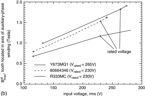
Figures E3.6.5a, E3.6.5b, E3.6.5c, and E3.6.5d show that the flux densities are approximately a linear function of the input voltage. In Figs. E3.6.6a and E3.6.6b comparison of the flux densities in the teeth and yoke (back iron) are presented for the methods discussed in the prior subsections of Section 3.7. The no-load currents of R333MC and 80664346 are depicted in Figs. E3.6.7a and E3.6.7b, respectively.


3.7.2.2 Discussion of Results and Conclusions
The permanent-split capacitor (PSC) motors of the air conditioners 80664346 and R333MC have the same output power and about the same overall dimensions (length and outer diameter). However, their stator and rotor windings are different. Measurements indicate that the 80664346 motor [36] generates a nearly sinusoidal flux density in the stator teeth (Fig. E3.6.4a), whereas that of the R333MC motor exhibits nonsinusoidal waveform although its (Bmt)max is smaller. In addition, the no-load current of the 80664346 (Fig. E3.6.7b) is about half that of R333MC (Fig. E3.6.7a), although the latter’s maximum flux density in stator teeth and back iron (yoke) is less (Figs. E3.6.4a and E3.6.4c). This indicates that the proper designs of the stator and rotor windings are important for the waveform of the stator tooth flux density and its associated iron-core loss, and for the efficiency optimization of PSC motors.
The yoke flux densities (Figs. E3.6.4b and E3.6.4d) are mostly sinusoidal for all machines tested [36]. Although 80664346 has a larger flux density than R333MC, the no-load losses of 80664346 are smaller as can be seen from their stator, rotor, and magnetizing parameters. References [30], [37], and Appendix of [38] address how time-dependent waveforms of the magnetizing current depend on the spatial distribution/pitch of a winding. Figures E3.6.5a through E3.6.5d show that in these three PSC motors saturation in stator teeth and yokes is small as compared to transformers, and therefore the principle of superposition with respect to flux densities and losses can be applied. Figures E3.6.6a and E3.6.6b demonstrate that both the computer sampling and the oscilloscope methods lead to similar results with respect to maximum flux densities. One concludes that although a single-phase motor (e.g., 80664346) has relatively large flux densities in stator yoke and teeth the no-load current can be relatively small, although it is quite nonsinusoidal. One of the reasons for this is that the power factor at no load is relatively large. The best design of a PSC motor is thus not necessarily based on sinusoidal current wave shapes. Further work should investigate the following:
• the losses generated by alternating flux densities as they occur in the stator teeth, and rotating flux densities as they occur in the stator yoke, and
• the interrelation between time and space harmonics and their effects on loss generation.