
3.8 Inter- and subharmonic torques of three-phase induction machines
In Sections 3.4 and 3.5 the magnetomotive forces (mmfs) of spatial and time harmonics including the fundamental fields were derived, respectively. It can be shown that harmonic fields (where h = integer) generate very small asynchronous torques as compared with the fundamental torque. Sub- and interharmonic (0 ≤ h ≤ 1) torques, however, can generate parasitic torques near zero speed – that is, during the start-up of an induction motor. The formulas derived for harmonic torques are valid also for sub- and interharmonic torques. The following subsections confirm that sub- and interharmonic torques can have relatively large amplitudes if they originate from constant-voltage sources and not from constant-current sources.
3.8.1 Subharmonic Torques in a Voltage-Source-Fed Induction Motor
The equivalent circuit of a voltage-source-fed induction motor is shown in Fig. 3.38a for the fundamental (h = 1) and for the harmonic of order h. Using Thevenin’s theorem (subscript TH), the magnetizing branch can be eliminated (Fig. 3.38b) and one obtains the following relation for the electrical torque of the hth harmonic where ![]()


The Thevenin-adjusted machine parameters are

with


The mechanical synchronous angular velocity is

where ω1 is the electrical synchronous angular velocity, p is the number of poles, and q1 is the number of phases (e.g., q1 = 3).
In order to obtain the maximum or breakdown torque one matches the impedances of the Thevenin-adjusted equivalent circuit at sh = shmax:

and the breakdown slip for the hth harmonic becomes

The maximum motoring (mot) positive torque and the maximum generator (gen) negative torque for the time harmonic of hth order are


The generator (gen) electrical torque reaches its absolute (abs) maximum, if
that is,

3.8.2 Subharmonic Torques in a Current-Source-Fed Induction Motor
The equivalent circuits of a current-source-fed induction motor are shown in Fig. 3.39a,b for the fundamental (h = 1) and for the harmonic of order h.

The torque of the hth time harmonic is, from Fig. 3.39b,

where ![]() .
.
The breakdown slip is
Two application examples will be presented where an induction motor is first fed by a voltage source and then by a current source containing a forward rotating subharmonic component of 6 Hz (h = 0.1).
3.8.3 Application Example 3.7: Computation of Forward-Rotating Subharmonic Torque in a Voltage-Source-Fed Induction Motor
Terminal voltages of a three-phase induction motor contain the forward-rotating subharmonic of 6 Hz at an amplitude of V0.1 = 5%. The fundamental voltage is V1 = 240 V and the parameters of a three-phase induction machine are as follows:

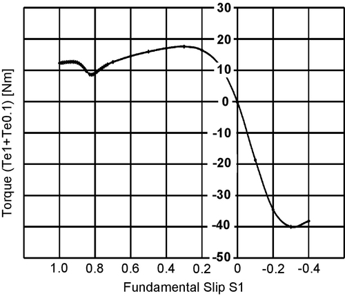
Compute and plot the sum of the fundamental and subharmonic torques (Te1 + Te0.1) as a function of the fundamental slip s1.
Solution to Application Example 3.7
Parameters of Eqs. 3-47 to 3-54 are listed as a function of the fundamental (h = 1) and subharmonic h = 0.1 in Table E3.7.1. Fundamental torque values Te1 are listed in Table E3.7.2 as a function of the fundamental slip s1.
Table E3.7.1
Maximum Torques for Fundamental (h = 1) and Subharmonic (h = 0.1) Voltages, where the Fundamental Voltage is 100% and the Subharmonic Voltage is 5% of the Fundamental Voltage
| h | VshTH (V) | ± Shmax (–) | ωmsh (rad/s) | Teh maxmot (Nm) | Teh maxgen (Nm) |
| 1 | 223.34 | 0.312 | 188.49 | 17.98 | –39.89 |
| 0.1 | 9.62 | 0.820 | 18.849 | 0.696 | –4.61 |

Table E3.7.2
Fundamental Torque Te1 as a Function of Fundamental Slip s1
| S1 (–) | 2.0 | 1.0 | 0.9 | 0.8 | 0.7 |
| Te1 (Nm) | 6.78 | 11.61 | 12.44 | 13.37 | 14.40 |
| S1 (–) | 0.6 | 0.5 | 0.4 | 0.3 | 0.2 |
| Te1 (Nm) | 15.5 | 16.63 | 17.59 | 17.97 | 16.76 |
| S1 (–) | 0.1 | 0.0344 | 0 | –0.1 | –0.2 |
| Te1 (Nm) | 11.8 | 4.99 | 0 | –18.46 | –34.32 |

The plot of the positively rotating fundamental torque characteristic Te1 = f(s1) is shown in Fig. E3.7.1 and the positively rotating torque Te0.1 = f(s0.1) is depicted in Fig. E3.7.2, where the 6 Hz voltage component has an amplitude of 5%, that is, V6Hz = 0.05 · V60Hz = 0.05(240 V) = 12 V.


Subharmonic torque values Te0.1 are listed in Table E3.7.3 as a function of the subharmonic slip s0.1.
Table E3.7.3
Subharmonic Torque Te0.1 as a Function of Subharmonic Slip s0.1
| S0.1 (–) | 1.0 | 0.9 | 0.82 | 0.8 | 0.7 | 0.6 |
| S1 (–) | 1.0 | 0.99 | 0.982 | 0.98 | 0.97 | 0.96 |
| Te0.1 (Nm) | 0.687 | 0.693 | 0.696 | 0.695 | 0.69 | 0.676 |
| S0.1 (–) | 0.5 | 0.4 | 0.3 | 0.2 | 0.1 | 0 |
| S1 (–) | 0.95 | 0.94 | 0.93 | 0.92 | 0.91 | 0.9 |
| Te0.1 (Nm) | 0.648 | 0.602 | 0.528 | 0.415 | 0.247 | 0 |
| S0.1 (–) | –0.1 | –0.2 | –0.3 | –0.4 | –0.5 | –0.6 |
| S1 (–) | 0.89 | 0.88 | 0.87 | 0.86 | 0.85 | 0.84 |
| Te0.1 (Nm) | –0.353 | –0.842 | –1.488 | –2.28 | –3.12 | –3.88 |
| S0.1 (–) | –0.7 | –0.8 | –0.82 | –0.9 | –1 | –1.1 |
| S1 (–) | 0.83 | 0.82 | 0.818 | 0.81 | 0.8 | 0.79 |
| Te0.1 (Nm) | –4.40 | –4.60 | –4.61 | –4.53 | –4.29 | –3.95 |
| S0.1 (–) | –1.2 | –1.3 | –1.4 | –1.5 | –1.6 | –1.7 |
| S1 (–) | 0.78 | 0.77 | 0.76 | 0.75 | 0.74 | 0.73 |
| Te0.1 (Nm) | –3.60 | –3.26 | –2.96 | –2.68 | –2.45 | –2.24 |
| S0.1 (–) | –2.0 | –3.0 | –4.0 | –5.0 | –6.0 | –7.0 |
| S1 (–) | 0.70 | 0.60 | 0.50 | 0.40 | 0.30 | 0.20 |
| Te0.1 (Nm) | –1.76 | –0.98 | –0.67 | –0.51 | –0.40 | –0.34 |
| S0.1 (–) | –8.0 | –9.0 | –10.0 | –11.0 | –12.0 | –13.0 |
| S1 (–) | 0.1 | 0 | –0.1 | –0.20 | –0.30 | –0.40 |
| Te0.1 (Nm) | –0.29 | –0.25 | –0.22 | –0.20 | –0.18 | –0.17 |

Using Eqs. 3-4d and 3-25 one can compute the fundamental torque Te1 and the subharmonic torque Te0.1 as a function of the fundamental slip s1 (Table E3.7.4). For example a subharmonic (h = 0.1) slip of s0.1 = 1 corresponds to a fundamental slip of (see Eqs. 3-31b, 3-32, and Table E3.7.3)
Table E3.7.4
Fundamental and Subharmonic Torque (Te1 + Te0.1) as a Function of Fundamental Slip s1
| S1 (–) | 1.0 | 0.99 | 0.982 | 0.98 | 0.97 | 0.96 |
| Te1 (Nm) | 11.61 | 11.69 | 11.75 | 11.77 | 11.85 | 11.93 |
| Te1 + Te0.1 (Nm) | 12.30 | 12.38 | 12.45 | 12.46 | 12.54 | 12.60 |
| S1 (–) | 0.95 | 0.94 | 0.93 | 0.92 | 0.91 | 0.9 |
| Te1 (Nm) | 12.01 | 12.10 | 12.18 | 12.27 | 12.35 | 12.44 |
| Te1 + Te0.1 (Nm) | 12.66 | 12.70 | 12.71 | 12.68 | 12.60 | 12.44 |
| S1 (–) | 0.89 | 0.88 | 0.87 | 0.86 | 0.85 | 0.83 |
| Te1 (Nm) | 12.53 | 12.62 | 12.71 | 12.80 | 12.89 | 13.08 |
| Te1 + Te0.1 (Nm) | 12.18 | 11.78 | 11.22 | 10.52 | 9.77 | 8.68 |
| S1 (–) | 0.82 | 0.818 | 0.81 | 0.8 | 0.79 | 0.78 |
| Te1 (Nm) | 13.18 | 13.19 | 13.27 | 13.37 | 13.47 | 13.57 |
| Te1 + Te0.1 (Nm) | 8.58 | 8.58 | 8.74 | 9.08 | 9.52 | 9.97 |
| S1 (–) | 0.77 | 0.76 | 0.75 | 0.74 | 0.73 | 0.70 |
| Te1 (Nm) | 13.67 | 13.77 | 13.87 | 13.97 | 14.08 | 14.40 |
| Te1 + Te0.1 (Nm) | 10.41 | 10.81 | 11.19 | 11.52 | 11.84 | 12.64 |
| S1 (–) | 0.60 | 0.50 | 0.40 | 0.30 | 0.20 | 0.10 |
| Te1 (Nm) | 15.50 | 16.63 | 17.59 | 17.97 | 16.76 | 11.80 |
| Te1 + Te0.1 (Nm) | 14.52 | 15.96 | 17.08 | 17.57 | 16.42 | 11.51 |
| S1 (–) | 0 | –0.10 | –0.20 | –0.30 | –0.40 | 0 |
| Te1 (Nm) | 0 | –18.46 | –34.32 | –39.84 | –38.01 | 0 |
| Te1 + Te0.1 (Nm) | –0.25 | –18.68 | –34.52 | –40.02 | –38.19 | 0 |

The plot of fundamental and subharmonic torque values (Te1 + Te0.1) as a function of fundamental slip (s1) is shown in Fig. E3.7.3.
3.8.4 Application Example 3.8: Rationale for Limiting Harmonic Torques in an Induction Machine
Based on results of the previous application example, explain why low-frequency subharmonic voltages at the terminal of induction machines should be limited.
Solution to Application Example 3.8
For subharmonic slip s0.1 = 1.0 one obtains with Eq. E3.7-2 the fundamental slip s1 = 1.0. Correspondingly for subharmonic slip s0.1 = 0.82 one obtains s1 = 0.982, and for subharmonic slip s0.1 = –0.82 one obtains s1 = 0.818 (see Table E3.7.3).
One notes that the subharmonic torque at 6 Hz (h = 0.1) is relatively large in the generator region (Te0.1 = –4.61 Nm). If the worst case is considered as defined by Eq. 3-52 the corresponding low-frequency harmonic torque is even larger. This is the reason why the low-frequency harmonic voltages should be limited to less than a few percent (e.g., 2%) of rated voltage.
3.8.5 Application Example 3.9: Computation of Forward-Rotating Subharmonic Torque in Current-Source-Fed Induction Motor
Terminal currents of a three-phase induction motor contain a forward-rotating subharmonic of 6 Hz at an amplitude I0.1 = 5% of the fundamental I1 = 1.73 A. The parameters of a three-phase induction machine are as follows:

Compute the fundamental torque (Te1) as a function of the fundamental slip (s1) and subharmonic torque (Te0.1) as a function of the subharmonic slip (s0.1).
Solution to Application Example 3.9
The parameters of Eqs. 3-53 and 3-54 and the corresponding fundamental and subharmonic torques are listed in Tables E3.9.1 through E3.9.3 as a function of the fundamental h = 1 and the subharmonic h = 0.1.
Table E3.9.1
Maximum Torques for Fundamental and Subharmonic Currents, where the Fundamental Current is 1.73 A and the Subharmonic Current is 5% of the Fundamental Current
| h | ± Shmax (–) | ωmsh (rad/s) | Teh maxmot (Nm) | Teh maxgen (Nm) | |
| 1 | 190.3 | 0.044 | 188.49 | 2.53 | –2.35 |
| 0.1 | 0.952 | 0.439 | 18.849 | 0.0063 | –0.0063 |

Table E3.9.2
Torque as a Function of Slip s1 for Fundamental (h = 1) Currents
| S1 (–) | 1.0 | 0.9 | 0.8 | 0.7 | 0.6 |
| Te1(Nm) | 0.221 | 0.246 | 0.276 | 0.316 | 0.368 |
| S1 (–) | 0.5 | 0.4 | 0.3 | 0.2 | 0.1 |
| Te1(Nm) | 0.440 | 0.548 | 0.724 | 1.058 | 1.860 |

Table E3.9.3
Torque as a Function of Slip s0.1 for Subharmonic (h = 0.1) Currents of 5% of the Fundamental Current
| S0.1 (–) | 1.0 | 0.9 | 0.8 | 0.7 | 0.6 |
| Te0.1 (Nm) | 0.0047 | 0.0050 | 0.0053 | 0.0057 | 0.0060 |
| S0.1 (–) | 0.5 | 0.4 | 0.3 | 0.2 | 0.1 |
| Te0.1 (Nm) | 0.0063 | 0.0063 | 0.0059 | 0.0048 | 0.0027 |

One notes that the low-frequency harmonic torques at 6 Hz and 5% harmonic current amplitudes are very small (about 0.0063 Nm).
3.9 Interaction of space and time harmonics of three-phase induction machines
For mmfs with a fundamental and a spatial harmonic of order H one obtains

where the currents consist of a fundamental and a time harmonic of order h:

In Eq. 3-55, A1, AH, θ, and H are fundamental mmf amplitude, harmonic mmf amplitude, mechanical (space) angular displacement, and spatial harmonic order, respectively. In Eq. 3-56, Im1, Imh, ω1, and h are fundamental current amplitude, harmonic current amplitude, electrical angular velocity, and (time) harmonic order, respectively. The total mmf becomes Ftotal = Fa + Fb + Fc ,

The evaluation of Eq. 3-57 depends on the amplitudes A1, AH, Im1, and Imh as well as on the harmonic orders h and H.
3.9.1 Application Example 3.10: Computation of Rotating MMF with Time and Space Harmonics
Compute the mmf and its angular velocities for an induction machine with the following time and space harmonics:
(a) A1 = 1 pu, AH = 0.05 pu, Im1 = 1 pu, Imh = 0.05 pu, H = 5, and h = 5.
(b) A1 = 1 pu, AH = 0.05 pu, Im1 = 1 pu, Imh = 0.05 pu, H = 13, and h = 0.5.
Solution to Application Example 3.10
a) For A1 = 1 pu, AH = 0.05 pu, Im1 = 1 pu, Imh = 0.05 pu, H = 5, and h = 5 one obtains the rotating mmf as
with the angular velocities

b) For A1 = 1 pu, AH = 0.05 pu, Im1 = 1 pu, Imh = 0.05 pu, H = 13, and h = 0.5 one obtains the rotating mmf as

with the angular velocities

3.9.2 Application Example 3.11: Computation of Rotating MMF with Even Space Harmonics
Nonideal induction machines may generate even space harmonics. For A1 = 1 pu, AH = 0.05 pu, Im1 = 1 pu, Imh = 0.05 pu, H = 12, and h = 0.1, compute the resulting rotating mmf and its angular velocities.
Solution to Application Example 3.11
with the angular velocities

3.9.3 Application Example 3.12: Computation of Rotating MMF with Noninteger Space Harmonics
Nonideal induction machines may generate noninteger space harmonics. For A1 = 1 pu, AH = 0.05 pu, Im1 = 1 pu, Imh = 0.05 pu, H = 13.5, and h = 0.1, compute the resulting rotating mmf and its angular velocities.
Solution to Application Example 3.12

with the angular velocities

Application Examples 3.10 to 3.12 illustrate how sub- and noninteger harmonics are generated by induction machines. Such harmonics may cause the malfunctioning of protective (e.g., under-frequency) relays within a power system [42].
The calculation of the asynchronous torques due to harmonics and inter- and subharmonics is based on the equivalent circuit without taking into account the variation of the differential leakage as a function of the numbers of stator slots and rotor slots. It is well known that certain stator and rotor slot combinations lead to asynchronous and synchronous harmonic torques in induction machines. A more comprehensive treatment of such parasitic asynchronous and synchronous harmonic torques is presented in [30,43–69]. Speed variation of induction motors is obtained either by voltage variation with constant frequency or by variation of the voltage and the fundamental frequency using inverters as a power source. Inverters have somewhat nonsinusoidal output voltages or currents. Thus parasitic effects like additional losses, dips in the torque–speed curve, output power derating, magnetic noise, oscillating torques, and harmonic line currents are generated. It has already been shown [43–45] that the multiple armature reaction has to be taken into account if effects caused by delta-connection of the stator windings, parallel winding branches, stator current harmonics, or damping of the air-gap field are to be considered. Moreover, the influence of the slot openings [46] and interbar currents [30,47,48,68] in case of slot skewing is important. Compared with conventional methods [25,30,68] the consideration of multiple armature reactions requires additional work consisting of the solution of a system of equations of the order from 14 to 30 for a three-phase induction machine and the summation of the air-gap inductances. The presented theory [69] is based on Fourier analysis and does not employ any transformation. As an alternative to the analytical method described [69] two-dimensional numerical methods (e.g., finite-element method) with time stepping procedures are available [49–51]. These have the advantages of analyzing transients, variable permeability, and eddy currents in solid iron parts, but have the disadvantages of grid generation, discretization errors, and preparatory work and require large computing CPU time.
3.10 Conclusions concerning induction machine harmonics
One can draw the following conclusions:
• Three-phase induction machines can generate asynchronous as well as synchronous torques depending on their construction (e.g., number of stator and rotor slots) and the harmonic content of their power supplies [25–69].
• The relations between harmonic slip sh and the harmonic slip referred to the fundamental slip sh(1) are the same for forward- and backward-rotating harmonic fields.
• Harmonic torques Teh (where h = integer) are usually very small compared to the rated torque Te1.
• Low-frequency and subharmonic torques (0 ≤ h ≤ 1) can be quite large even for small low-frequency and subharmonic voltage amplitudes (e.g., 5% of fundamental voltage). These low-frequency or subharmonics may occur in the power system or at the output terminals of voltage-source inverters.
• Low-frequency and subharmonic torques (0 ≤ h ≤ 1) are small even for large low-frequency harmonic current amplitudes (e.g., 5% of fundamental current) as provided by current sources.
• References [25], [28], and [39–41] address the heating of induction machines due to low-frequency and subharmonics, and reference [42] discusses the influence of inter- and subharmonics on under-frequency relays, where the zero crossing of the voltage is used to sense the frequency. Because of these negative influences the low-frequency, inter- and subharmonic voltage amplitudes generated in the power system due to inter- and subharmonic currents must be limited to below 0.1% of the rated voltage.
• Time and spatial harmonic voltages or currents may generate sufficiently large mmfs to cause significant harmonic torques near zero speed.
• The interaction of time and space harmonics generates sufficiently small mmfs so that start-up of an induction motor will not be affected.
3.11 Voltage-stress winding failures of ac motors fed by variable-frequency, voltage- and current-source pwm inverters
Motor winding failures have long been a perplexing problem for electrical engineers. There are a variety of different causes for motor failure: heat, vibration, contamination, defects, and voltage stress. Most of these are understood and can be controlled to some degree by procedure and/or design. Voltage (stress) transients, however, have taken on a new dimension with the development of variable-frequency converters (VFCs), which appear to be more intense than voltage stress on the motor windings caused by motor switching or lightning. This section will use induction motors as the baseline for explaining this phenomenon. However, it applies to transformers and synchronous machines as well.
Control and efficiency advantages of variable-frequency drives (VFDs) based on power electronic current- or voltage-source inverters lead to their prolific employment in utility power systems. The currents and voltages of inverters are not ideally sinusoidal but have small current ripples that flow in cables, transformers, and motor or generator windings. As a result of cable capacitances and parasitic capacitances this may lead to relatively large voltage spikes (see Application Example 3.14). Most short-circuits are caused by a breakdown of the insulation and thus are initiated by excessive voltage stress over some period of time. This phenomenon must be analyzed using traveling wave theory because the largest voltage stress does not necessarily appear at the input terminal but can occur because of the backward (reflected) traveling wave somewhere between the input and output terminals. An analysis of this phenomenon involving PWM inverters has not been done, although some engineers have identified this problem [70–74]. It is important to take into account the damping (losses) within the cables, windings, and cores because the voltage stress caused by the repetitive nature of PWM depends on the superposition of the forward-and backward-traveling waves, the local magnitudes of which are dependent on the damping impedances of the cable, winding, and core.
With improved semiconductor technology in VFDs and pulse-width modulators, the low-voltage induction motor drive has become a very viable alternative to the DC motor drive for many applications. The performance improvement, along with its relatively low cost, has made it a major part of process control equipment throughout the industry. The majority of these applications are usually under the 2 kV and the 1 MW range. Even with advancements in technology, the low-voltage induction motor experiences failures in the motor winding. Although there are differences between medium-voltage and high- and low-voltage induction motor applications, there are similarities between their failures.
The medium-voltage induction motor [75] experiences turn-to-turn failures when exposed to surge transients induced by switching or lightning. Most research shows that the majority of failures that occur in the last turn of the first coil prior to entering the second coil of the windings are due to (capacitor) switching transients. One might not expect to see turn-to-turn failures in small induction machines because of their relatively low voltage levels compared to their high insulation ratings, but this is not the case. Turn-to-turn failures are being experienced in all turns of the first coil of the motor.
As indicated above, most short-circuits in power systems occur because of insulation failure. The breakdown of the insulation depends on the voltage stress integrated over time. Although the time component cannot be influenced, the voltage stress across a dielectric can be reduced. Some preliminary work has been done in exploring this wave-propagation phenomenon where forward- and backward- traveling waves superimpose; here, the maximum voltage stress does not necessarily occur at the terminal of a winding, but somewhere in between the two (input, output) terminals. Because of the repetitive nature of PWM pulses, the damping due to losses in the winding and iron core cannot be neglected. The work by Gupta et al. [75] and many others [70–74,76–78] neglects the damping of the traveling waves; therefore, it cannot predict the maximum voltage stress of the winding insulation. Machine, transformer windings, and cables can be modeled by leakage inductances, resistances, and capacitances. Current-source inverters generate the largest voltage stress because of their inherent current spikes resulting in a large voltage L(di/dt).
The current model [75] of medium-voltage induction motors is based on the transmission line theory neglecting damping effects in windings and cores: since the turns of the coil are in such close proximity to each other, they form sections of a transmission line. As a single steep front wave, or surge, travels through the coil’s turns, it will encounter impedance mismatches, usually at the entrance and exit terminals of the coil, as well as at the transitions of the uniform parts (along the machine axial length) to the end winding parts. At these points of discontinuity, the wave will go through a transition, where it can be increased up to 2 per unit. With repetitive PWM pulses this is not the case: simulations have shown voltage increases to be as high as 20 times its source (rated) value due to the so-called swing effect. These increases in magnitude cause turn-to-turn failures in the windings. In dealing with medium-voltage induction motors [75], the transmission line theory neglecting any damping has been quite accurate in predicting where the failures are occurring for a single-current surge. This is not the case with low- and high-voltage induction motors fed by VFDs.
Existing theoretical results can be summarized as follows:
• The existing model [75–78] based on transmission line theory neglects the damping in the winding and iron core and, therefore, is not suitable for repetitive PWM switching simulation where the swing effect (cumulative increase of voltage magnitudes because of repetitive switching such that a reinforcement occurs due to positive feedback caused by winding parameter discontinuities) becomes important.
• A new equivalent circuit of induction motors based on a modified transmission line theory employing resistances, coupling capacitances, and inductances including the feeding cable has been developed, as is demonstrated in the following examples.
• The case of lossless transmission line segments modeling one entire phase of an induction motor with a single-current pulse for input agrees with the findings of the EPRI study [75] and other publications [76–78].
• Forward- and backward-traveling waves superimpose and generate different voltage stresses in coils. Voltage stresses will be different at different locations in the winding.
• Voltage stress appears to be dependent on PWM switching frequency, duty cycle, and motor parameters.
• Voltage stress is also dependent on the wave shape of the voltage/current surge. The wave shape is characterized by the rise, fall, and duration times as well as switching frequency.
• Current-source inverters (CSIs) produce larger voltage stress than voltage-source inverters (VSIs).
• Filters intended to reduce transient voltage damage to a motor may not be able to cover the entire frequency range of the inverter for a variable-frequency drive (VFD).
• Increases in voltage magnitude cause turn-to-turn and coil-to-frame failures in the windings.
• Increasing insulation at certain portions of a turn will help.
• Motor winding parameters are somewhat nonuniform due to the deep motor slots. Inductance and capacitance change along the coil (e.g., the end and slot regions of the coil).
3.11.1 Application Example 3.13: Calculation of Winding Stress Due to PMW Voltage-Source Inverters
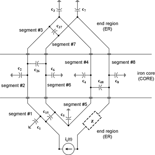
Voltage ripples due to PWM voltage-source inverters cause voltage stress in windings of machines and transformers. The configuration of Fig. E3.13.1 represents a simple winding with two turns consisting of eight segments. Each segment can be represented by an inductance Li, a resistance Ri, and a capacitance to ground (frame) Ci, and there are four interturn capacitances Cij and inductances Lij. Figure E3.13.2 represents a detailed equivalent circuit for the configuration of Fig. E3.13.1.


a) To simplify the analysis neglect the capacitances Cij and the inductances Lij. This leads to the circuit of Fig. E3.13.3, where the winding is fed by a PWM voltage source (see Fig. E3.13.4). One obtains the 16 differential equations (Eqs. E3.13-1a,b to E3.13-8a,b) as listed below.


The parameters are
R1 = R2 = R3 = R4 = R5 = R6 = R7 = R8 = 25 μΩ;
L1 = L3 = L5 = L7 = 1 mH, L2 = L4 = L6 = L8 = 10 mH;
C1 = C3 = C5 = C7 = 0.7 pF, C2 = C4 = C6 = C8 = 7 pF,
C15 = C37 = 0.35 pF, C26 = C48 = 3.5 pF;
G1 = G3 = G5 = G7 = 1/(5000 Ω),
G2 = G4 = G6 = G8 = 1/(500 Ω); L15 = L37 = 0.005 mH,
L26 = L48 = 0.01 mH.
Z is either 1 μΩ (short-circuit) or 1 MΩ (open-circuit). As input, assume the PWM voltage-step function vs(t) (illustrated in Fig. E3.13.4).
Using Mathematica or MATLAB compute all state variables for the time period from t = tcalculate = 0 to 2.1 ms. Note that for some reason tcalculate must be larger than tplot. Plot the voltages (vs – v1), (v1 – v5), (v2 – v6), (v3 – v7), and (v4 – v8).
b) For the detailed equivalent circuit of Fig. E3.13.2 establish all differential equations in a similar manner as has been done in part a. As input, assume a PWM voltage-step function vs(t) (illustrated in Fig. E3.13.4).
Solution to Application Example 3.13
Solution #1 (Based on Mathematica)
a) Program list for short circuit with Z = 10- 6Ω is presented in Table E3.13.1 and the cooresponding plots are shown in Figs. E3.13.5 to E3.13.10. Note that the computing time t = tcalculate = 2.1 ms must be larger than the plot time t = tplot = 2 ms.
Program list for open circuit with Z = 106Ω is presented in Table E3.13.2 and the cooresponding plots are shown in Figs. E3.13.11 to E3.13.15. Note that the computing time t = tcalculate = 2.1 ms must be larger than the plot time t = tplot = 2 ms.
Table E3.13.1
Mathematica program list for Application Example 3.13 (part a) for short- circuit with Z = 10- 6Ω
| Hval = 10.01; Lval = 0; period = 200*10ˆ-6; duty = 0.5; Vs[t_]:=If[Mod[t,period] < duty*period,Hval,Lval]; Plot[Vs[t],{t,0,0.001},PlotRange- > All,AxesLabel - > {“t(s)”,“Vs(t)”}] R1 = 25*10ˆ-6; | eq1 = I1'[t]==-R1/L1*I1[t]-V1[t]/L1 + Vs[t]/L1; ic1 = I1[0]==0; eq2 = V1'[t]==I1[t]/C1-G1/C1*V1[t]-I2[t]/C1; ic2 = V1[0]==0; eq3 = I2'[t]==-R2/L2*I2[t]-V2[t]/L2 + V1[t]/L2; ic3 = I2[0]==0; eq4 = V2'[t]==I2[t]/C2-G2/C2*V2[t]-I3[t]/C2; ic4 = V2[0]==0; eq5 = I3'[t]==-R3/L3*I3[t]-V3[t]/L3 + V2[t]/L3; ic5 = I3[0]==0; |
| R2 = 25*10ˆ-6; R3 = 25*10ˆ-6; R4 = 25*10ˆ-6; R5 = 25*10ˆ-6; R6 = 25*10ˆ-6; R7 = 25*10ˆ-6; R8 = 25*10ˆ-6; L1 = 1*10ˆ-3; L3 = 1*10ˆ-3; L5 = 1*10ˆ-3; L7 = 1*10ˆ-3; L2 = 10*10ˆ-3; L4 = 10*10ˆ-3; L6 = 10*10ˆ-3; L8 = 10*10ˆ-3; L15 = 5*10ˆ-6; L37 = 5*10ˆ-6; L26 = 10*10ˆ-6; L48 = 10*10ˆ-6; C1 = .7*10ˆ-12; C3 = .7*10ˆ-12; C5 = .7*10ˆ-12; C7 = .7*10ˆ-12; C2 = 7*10ˆ-12; C4 = 7*10ˆ-12; C6 = 7*10ˆ-12; C8 = 7*10ˆ-12; C15 = .35*10ˆ-12; C37 = .35*10ˆ-12; C26 = 3.5*10ˆ-12; C48 = 3.5*10ˆ-12; G1 = 1/5000; G3 = 1/5000; G5 = 1/5000; G7 = 1/5000; G2 = 1/500; G4 = 1/500; G6 = 1/500; G8 = 1/500; Z = 1*10ˆ-6; | eq6 = V3'[t]==I3[t]/C3-G3/C3*V3[t]-I4[t]/C3; ic6 = V3[0]==0; eq7 = I4'[t]==-R4/L4*I4[t]-V4[t]/L4 + V3[t]/L4; ic7 = I4[0]==0; eq8 = V4'[t]==I4[t]/C4-G4/C4*V4[t]-I5[t]/C4; ic8 = V4[0]==0; eq9 = I5'[t]==-R5/L5*I5[t]-V5[t]/L5 + V4[t]/L5; ic9 = I5[0]==0; eq10 = V5'[t]==I5[t]/C5-G5/C5*V5[t]-I6[t]/C5; ic10 = V5[0]==0; eq11 = I6'[t]==-R6/L6*I6[t]-V6[t]/L6 + V5[t]/L6; ic11 = I6[0]==0; eq12 = V6'[t]==I6[t]/C6-G6/C6*V6[t]-I7[t]/C6; ic12 = V6[0]==0; eq13 = I7'[t]==-R7/L7*I7[t]-V7[t]/L7 + V6[t]/L7; ic13 = I7[0]==0; eq14 = V7'[t]==I7[t]/C7-G7/C7*V7[t]-I8[t]/C7; ic14 = V7[0]==0; eq15 = I8'[t]==−R8/L8*I8[t]/L8+V7[t]/L8; ic15 = I8[0]==0; eq16 = V8'[t]==I8[t]/C8-V8[t]*(1/(Z*C8) + G8/C8); ic16 = V8[0]==0; sol1 = NDSolve[{eq1,eq2,eq3,eq4,eq5,eq6,eq7, eq8,eq9,eq10,eq11,eq12,eq13,eq14,eq15,eq16, ic1,ic2,ic3,ic4,ic5,ic6,ic7,ic8,ic9,ic10,ic11,ic12, ic13,ic14,ic15,ic16},{I1[t],V1[t],I2[t],V2[t],I3[t], V3[t],I4[t],V4[t],I5[t],V5[t],I6[t],V6[t],I7[t],V7[t], I8[t],V8[t]},{t,0,0.0022},MaxSteps- > 100000]; Plot[Vs[t]-Evaluate[V1[t]/.sol1],{t,0,0.002}, AxesLabel- > {“Time”, “(Vs-V1) (V)”}] Plot[Evaluate[V1[t]/.sol1]-Evaluate[V5[t]/.sol1], {t,0,0.002},AxesLabel- > {“t(s)”, “(V1-V5) (V)”}] Plot[Evaluate[V2[t]/.sol1]-Evaluate[V6[t]/.sol1], {t,0,0.002},AxesLabel- > {“t(s)”, “(V2-V6) (V)”}] Plot[Evaluate[V3[t]/.sol1]-Evaluate[V7[t]/.sol1], {t,0,0.002},AxesLabel- > {“t(s)”, “(V3-V7) (V)”}] Plot[Evaluate[V4[t]/.sol1]-Evaluate[V8[t]/.sol1], {t,0,0.002},AxesLabel- > {“t(s)”, “(V4-V8) (V)”}] |


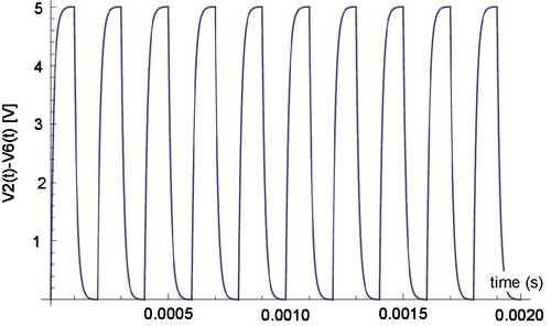


Table E3.13.2
Mathematica program list for Application Example 3.13 (part a) for open- circuit with Z = 106Ω
| Hval = 10.; Lval = 0; period = 200*10ˆ-6; duty = 0.5; Vs[t_]:=If[Mod[t,period] < duty*period,Hval,Lval]; Plot[Vs[t],{t,0,0.001},PlotRange- > All,AxesLabel - > {“t(s)”,“Vs(t)”}] R1 = 25*10ˆ-6; R2 = 25*10ˆ-6; R3 = 25*10ˆ-6; R4 = 25*10ˆ-6; R5 = 25*10ˆ-6; R6 = 25*10ˆ-6; R7 = 25*10ˆ-6; R8 = 25*10ˆ-6; L1 = 1*10ˆ-3; L3 = 1*10ˆ-3; L5 = 1*10ˆ-3; L7 = 1*10ˆ-3; L2 = 10*10ˆ-3; L4 = 10*10ˆ-3; L6 = 10*10ˆ-3; L8 = 10*10ˆ-3; L15 = 5*10ˆ-6; L37 = 5*10ˆ-6; L26 = 10*10ˆ-6; L48 = 10*10ˆ-6; C1 = .7*10ˆ-12; C3 = .7*10ˆ-12; C5 = .7*10ˆ-12; C7 = .7*10ˆ-12; C2 = 7*10ˆ-12; C4 = 7*10ˆ-12; C6 = 7*10ˆ-12; C8 = 7*10ˆ-12; C15 = .35*10ˆ-12; C37 = .35*10ˆ-12; | eq1 = I1'[t]==-R1/L1*I1[t]-V1[t]/L1 + Vs[t]/L1; ic1 = I1[0]==0; eq2 = V1'[t]==I1[t]/C1-G1/C1*V1[t]-I2[t]/C1; ic2 = V1[0]==0; eq3 = I2'[t]==-R2/L2*I2[t]-V2[t]/L2 + V1[t]/L2; ic3 = I2[0]==0; eq4 = V2'[t]==I2[t]/C2-G2/C2*V2[t]-I3[t]/C2; ic4 = V2[0]==0; eq5 = I3'[t]==-R3/L3*I3[t]-V3[t]/L3 + V2[t]/L3; ic5 = I3[0]==0; eq6 = V3'[t]==I3[t]/C3-G3/C3*V3[t]-I4[t]/C3; ic6 = V3[0]==0; eq7 = I4'[t]==-R4/L4*I4[t]-V4[t]/L4 + V3[t]/L4; ic7 = I4[0]==0; eq8 = V4'[t]==I4[t]/C4-G4/C4*V4[t]-I5[t]/C4; ic8 = V4[0]==0; eq9 = I5'[t]==-R5/L5*I5[t]-V5[t]/L5 + V4[t]/L5; ic9 = I5[0]==0; eq10 = V5'[t]==I5[t]/C5-G5/C5*V5[t]-I6[t]/C5; ic10 = V5[0]==0; eq11 = I6'[t]==-R6/L6*I6[t]-V6[t]/L6 + V5[t]/L6; ic11 = I6[0]==0; eq12 = V6'[t]==I6[t]/C6-G6/C6*V6[t]-I7[t]/C6; ic12 = V6[0]==0; eq13 = I7'[t]==-R7/L7*I7[t]-V7[t]/L7 + V6[t]/L7; ic13 = I7[0]==0; eq14 = V7'[t]==I7[t]/C7-G7/C7*V7[t]-I8[t]/C7; ic14 = V7[0]==0; eq15 = I8'[t]==-R8/L8*I8[t]-V8[t]/L8 + V7[t]/L8; ic15 = I8[0]==0; eq16 = V8'[t]==I8[t]/C8-V8[t]*(1/(Z*C8) + G8/C8); ic16 = V8[0]==0; sol1 = NDSolve[{eq1,eq2,eq3,eq4,eq5,eq6,eq7,eq8, eq9,eq10,eq11,eq12,eq13,eq14,eq15,eq16,ic1,ic2, ic3,ic4,ic5,ic6,ic7,ic8,ic9,ic10,ic11,ic12,ic13,ic14, ic15,ic16},{I1[t],V1[t],I2[t],V2[t],I3[t],V3[t],I4[t], V4[t],I5[t],V5[t],I6[t],V6[t],I7[t],V7[t],I8[t],V8[t]} ,{t,0,0.0022},MaxSteps- > 100000]; Plot[Vs[t]-Evaluate[V1[t]/.sol1],{t,0,0.002}, |
| C26 = 3.5*10ˆ-12; C48 = 3.5*10ˆ-12; G1 = 1/5000; G3 = 1/5000; G5 = 1/5000; G7 = 1/5000; G2 = 1/500; G4 = 1/500; G6 = 1/500; G8 = 1/500; Z = 1*10ˆ6; | AxesLabel- > {“Time”, “(Vs-V1) (V)”}] Plot[Evaluate[V1[t]/.sol1]-Evaluate[V5[t]/.sol1], {t,0,0.002},AxesLabel- > {“t(s)”,“(V1-V5) (V)”}] Plot[Evaluate[V2[t]/.sol1]-Evaluate[V6[t]/.sol1], {t,0,0.002},AxesLabel- > {"t(s)","(V2-V6) (V)"}] Plot[Evaluate[V3[t]/.sol1]-Evaluate[V7[t]/.sol1], {t,0,0.002},AxesLabel- > {“t(s)”,“(V3-V7) (V)”}] Plot[Evaluate[V4[t]/.sol1]-Evaluate[V8[t]/.sol1], {t,0,0.002},AxesLabel- > {“t(s)”,“(V4-V8) (V)”}] |


b) The detailed equivalent circuit (Fig. E3.13.2) generates about the same result as the simplified equivalent circuit (Fig. E3.13.3) and the results are therefore not given. Note, the state-variable equations of Eqs. E13-1 to E13-8 are still valid for the detailed equivalent circuit. However, the following four equations need to be added (assuming that the initial current through all the branches is zero):


Solution #2 (Based on MATLAB)
The results as obtained from Mathematica and Matlab are not exactly identical due to the different intergration algorithms used by both software programs, and the results are not given here due to space limitations.
3.11.2 Application Example 3.14: Calculation of Winding Stress Due to PMW Current-Source Inverters
Current ripples due to PWM current-source inverters cause voltage stress in windings of machines and transformers. The configuration of Fig. E3.14.1 represents a simple winding with two turns. Each winding can be represented by four segments having an inductance Li, a resistance Ri, a capacitance to ground (frame) Ci, and some interturn capacitances Cij and inductances Lij. Figure E.3.14.2 represents a detailed equivalent circuit for the configuration of Fig. E3.14.1.


a) To simplify the analysis neglect the capacitances Cij and the inductances Lij. This leads to the circuit of Fig. E3.14.3, where the winding is fed by a PWM current source. One obtains the 15 differential equations of Eqs. E3.14-1 to E3.14-8a,b as listed below. In this case the current through L1 is given (e.g., is(t)) and, therefore, there are only 15 differential equations, as compared with Application Example 3.13.


The parameters are
R1 = R2 = R3 = R4 = R5 = R6 = R7 = R8 = 25 μΩ;
L1 = L3 = L5 = L7 = 1 mH, L2 = L4 = L6 = L8 = 10 mH;
C1 = C3 = C5 = C7 = 0.7 pF, C2 = C4 = C6 = C8 = 7 pF,
C15 = C37 = 0.35 pF, C26 = C48 = 3.5 pF;
G1 = G3 = G5 = G7 = 1/(5000 Ω),
G2 = G4 = G6 = G8 = 1/(500 Ω); and
L15 = L37 = 0.005 mH, L26 = L48 = 0.01 mH.
Z is either 1 μΩ (short-circuit) or 1 MΩ (open-circuit). Assume a PWM current-step function is(t) as indicated in Fig. E3.14.4.

b) For the simplified equivalent circuit using Mathematica compute all state variables during the time period from t = tcalculate = 0 to 2.1 ms at rise times of trise = 5 μs and 75 μs. Plot the current is (t) for 1 ms and voltages (v1 – v5), (v2 – v6), (v3 – v7), and (v4 – v8) for tplot = 2 ms.
Solution to Application Example 3.14
To demonstrate the sensitivity of the induced voltage stress as a function of the rise time of the current ripple, a rise time of 5 μs has been assumed first and the results based on Table E3.14.1 are plotted in Figs. E3.14.5 to E3.14.9 for Z = 10- 6Ω, that is the considered winding is short-circuited. Note, the voltage across capacitance C15 (that is, the voltage between the first turn and the second turn at the end region (ER)) is very large. For trise = 75 μs at Z =10- 6Ω the voltage stress is smaller (see Figs. E3.14.10 to E3.14.14).
Table E3.14.1
Mathematica program list for Application Example 3.13 (part a) for short- circuit with Z = 10- 6Ω
| amp = 5; period = 200*ˆ-6; duty = 0.5; trise = 5*Λ-6; Is[t_]:=If[Mod[t,period] > duty*period, 0,If[Mod[t,period] < trise,amp/(trise) *Mod[t,period],amp-amp/(period*duty-trise) *(Mod[t,period]-trise)]]; | ic6 = V3[0]==0; eq7 = I4’[t]==–R4/L4*I4[t]–V4[t]/L4 + V3[t]/L4; ic7 = I4[0]==0; eq8 = V4’[t]==I4[t]/C4–G4/C4*V4[t]–I5[t]/C4; ic8 = V4[0]==0; eq9 = I5’[t]==–R5/L5*I5[t]–V5[t]/L5 + V4[t]/L5; ic9 = I5[0]==0; eq10 = V5’[t]==I5[t]/C5–G5/C5*V5[t]-I6[t]/C5; ic10 = V5[0]==0; eq11 = I6’[t]==–R6/L6*I6[t]-V6[t]/L6 + V5[t]/L6; |
| Plot[Is[t],{t,0,.001},PlotRange → All,AxesLabel →{“t”,”Is(t)”}] R1 = 25*ˆ–6; R2 = 25*ˆ–6; R3 = 25*ˆ–6; R4 = 25*ˆ–6; R5 = 25*ˆ–6; R6 = 25*ˆ–6; R7 = 25*ˆ–6; R8 = 25*ˆ–6; L1 = 1*ˆ–3; L3 = 1*ˆ–3; L5 = 1*ˆ–3; L7 = 1*ˆ–3; L2 = 10*ˆ–3; L4 = 10*ˆ–3; L6 = 10*ˆ–3; L8 = 10*ˆ–3; L15 = 5*ˆ–6; L37 = 5*ˆ–6; L26 = 10*ˆ–6; L4 8 = 10*ˆ–6; C1 = .7*ˆ–12; C3 = .7*ˆ–12; C5 = .7*ˆ–12; C7 = .7*ˆ–12; C2 = 7*ˆ–12; C4 = 7*ˆ–12; C6 = 7*ˆ–12; C8 = 7*ˆ–12; C15 = .35*ˆ–12; C37 = .35*ˆ–12; C26 = 3.5*ˆ–12; C48 = 3.5*ˆ–12; G1 = 1/5000; G3 = 1/5000; G5 = 1/5000; G7 = 1/5000; G2 = 1/500; G4 = 1/500; G6 = 1/500; G8 = 1/500; Z = 1*ˆ–6; eq2 = V1’[t]==Is[t]/C1–G1/C1*V1[t]–I2[t]/C1; ic2 = V1[0]==0; eq3 = I2’[t]==–R2/L2*I2[t]–V2[t]/L2 + V1[t]/L2; ic3 = I2[0]==0; eq4 = V2’[t]==I2[t]/C2–G2/C2*V2[t]–I3[t]/C2; ic4 = V2[0]==0; eq5 = I3’[t]==–R3/L3*I3[t]–V3[t]/L3 + V2[t]/L3; ic5 = I3[0]==0; eq6 = V3’[t]==I3[t]/C3–G3/C3*V3[t]–I4[t]/C3; | ic11 = I6[0]==0; eq12 = V6’[t]==I6[t]/C6–G6/C6*V6[t]–I7[t]/C6; ic12 = V6[0]==0; eq13 = I7’[t]==–R7/L7*I7[t]–V7[t]/L7 + V6[t]/L7; ic13 = I7[0]==0; eq14 = V7’[t]==I7[t]/C7–G7/C7*V7[t]–I8[t]/C7; ic14 = V7[0]==0; eq15 = I8’[t]==–R8/L8*I8[t]–V8[t]/L8 + V7[t]/L8; ic15 = I8[0]==0; eq16 = V8’[t]==I8[t]/C8–V8[t]*(1/(Z*C8) + G8/C8); ic16 = V8[0]==0; sol1 = NDSolve[{eq2,eq3,eq4,eq5,eq6,eq7,eq8,eq9, eq10,eq11,eq12,eq13,eq14,eq15,eq16,ic2,ic3,ic4,ic5, ic6,ic7,ic8,ic9,ic10,ic11,ic12,ic13,ic14,ic15,ic16}, {V1[t],I2[t],V2[t],I3[t],V3[t],I4[t],V4[t],I5[t],V5[t],I6[t], V6[t],I7[t],V7[t],I8[t],V8[t]},{t,0,.002},MaxSteps → 100000] Plot[Evaluate[V1[t]/.sol1]−Evaluate[V5[t]/.sol1],{t,0,.002}, AxesLabel → {“Time”, “V1 – V5”}] Plot[Evaluate[V2[t]/.sol1] –Evaluate[V6[t]/.sol1],{t,0,.002}, AxesLabel → {“Time”, “V2 – V6”}] Plot[Evaluate[V3[t]/.sol1] –Evaluate[V7[t]/.sol1],{t,0,.002}, AxesLabel → {“Time”, “V3 – V7”}] Plot[Evaluate[V4[t]/.sol1] –Evaluate[V8[t]/.sol1],{t,0,.002}, AxesLabel → {“Time”, “V4 – V8”}] |


The voltage stresses at open circuit (Z = 106 Ω) at a rise time of trise =15 μs and 75 μs are similar to those of Figures E3.14.5 to E3.14.14.
Conclusions with respect to voltage stresses as investigated in Application Examples #3.13 and 3.14
1) The impedance Z (either short-circuit (10- 6 Ω) or open-circuit (106 Ω) coils) and the rectangular voltage sources vs(t) of Figure E3.13.5 — caused by ripples due to voltage-source PWM switching—do not generate large voltage stresses, for example v1(t)- v5(t) as shown in Figure E3.13.7 with a peak value of about 9 V.
2) The impedance Z (either short-circuit (10- 6 Ω) or open-circuit (106 Ω) coils) and the triangular current source is(t) with a risetime of trise = 5 μs of Figure E3.14.5 — caused by ripples due to current-source PWM switching--do generate very large voltage stresses, for example v1(t)- v5(t) as shown in Figure E3.14.6 with a peak value of about 10 k V.
3) The impedance Z (either short-circuit (10- 6 Ω) or open-circuit (106 Ω) coils) and the triangular current source is(t) with a risetime of trise = 75 μs of Figure E3.14.10 -- caused by ripples due to current-source PWM switching--do generate large voltage stresses, for example v1(t)- v5(t) as shown in Figure E3.14.11 with a peak value of about -2700 V.
3.12 Nonlinear harmonic models of three-phase induction machines
The aim of this section is to introduce and briefly discuss some harmonic models for induction machines available in the literature. Detailed explanations are given in the references cited.
3.12.1 Conventional Harmonic Model of an Induction Motor
Figures 3.3 and 3.25 represent the fundamental and harmonic per-phase equivalent circuits of a three-phase induction motor, respectively, which are used for the calculation of the steady-state performance. The rotor parameters may consist of the equivalent rotor impedance taking into account the cross-path resistance of the rotor winding, which is frequency dependent because of the skin effect in the rotor bars. The steady-state performance is calculated by using the method of superposition based on Figs. 3.3 and 3.25. In general, for the usual operating speed regions, the fundamental slip is very small and, therefore, the harmonic slip, sh, is close to unity.
3.12.2 Modified Conventional Harmonic Model of an Induction Motor
In order to improve the loss prediction of the conventional harmonic equivalent circuit of induction machines (Fig. 3.25), the core loss and stray-core losses associated with high-frequency leakage fluxes are taken into account. Stray-load losses in induction machines are considered to be important – due to leakage – when induction machines are supplied by nonsinusoidal voltage or current sources. This phenomenon can be accounted for by a modified loss model, as shown in Fig. 3.40 [79].

Inclusion of Rotor-Core Loss
Most publications assume negligible rotor-core losses due to the very low frequency (e.g., slip frequency) of the magnetic field within the rotor core. To take into account the rotor-iron losses – associated with the magnetizing path – a slip-dependent resistance R′mh is connected in parallel with the stator-core loss resistance (Fig. 3.40).
Iron Loss Associated with Leakage Flux Paths (Harmonic Stray Loss)
Resistances in parallel with the primary and the secondary leakage inductances (Rlsh, R′lrh) in the harmonic equivalent circuit of Fig. 3.40 represent harmonic losses, referred to as stray losses. Because almost all stray losses result from hysteresis and eddy-current effects, these equivalent parallel resistors are assumed to be frequency dependent.
3.12.3 Simplified Conventional Harmonic Model of an Induction Motor
As the mechanical speed is very close to the synchronous speed, the rotor slip with respect to the harmonic mmfs will be close to unity (e.g., about 6/5 and 6/7 for the 5th and 7th harmonics, respectively). Therefore, the resistance (1 – sh)R′r/sh will be negligibly small in the harmonic model of Fig. 3.25, and the equivalent harmonic circuit may be reduced to that of Fig. 3.41. Only the winding resistances and the leakage inductances are included; the magnetizing branches are ignored because the harmonic voltages can be assumed to be relatively small, and at harmonic frequencies the core-flux density is small as well as compared with fundamental flux density. It should be noted that the winding resistances and leakage inductances are frequency dependent.

3.12.4 Spectral-Based Harmonic Model of an Induction Machine with Time and Space Harmonics
Figure 3.42 shows a harmonic equivalent circuit of an induction machine that models both time and space harmonics [81]. The three windings may or may not be balanced as each phase has its own per phase resistance Requj, reactance Xequj, and speed-dependent complex electromagnetic force emf Ẽj (where j = 1, 2, 3 represents the phase number). To account for the core losses, two resistances in parallel are added to each phase: Rc1 representing the portion of losses that depends only on phase voltages and (ωb/ωs)Rc2 representing losses that depend on the frequency and voltage of the stator (ωb is the rated stator frequency whereas ωs is the actual stator frequency).

To account for space-harmonic effects, the spectral approach modeling technique is used. This concept combines effects of time harmonics (from the input power supply) and space harmonics (from machine windings and magnetic circuits), bearing in mind that no symmetrical components exist in both quantities.
The equivalent circuit of Fig. 3.42 has several branches (excluding the fundamental and the core losses), where each branch per phase is associated with one harmonic of the power supply (impedance) or one frequency for the space distribution (current source). To evaluate various parameters, the spectral analysis of both time-domain stator voltages and currents are required. The conventional blocked-rotor, no-load, and loaded shaft tests can be performed at fundamental frequency to evaluate phase resistance Requj, reactance Xequj, complex emf Ẽj, Rc1, and Rc2.
The harmonic stator voltage (![]() fij) and current (Ĩfij) with their respective magnitudes and phase angles need to be measured to determine harmonic impedances (e.g., Rfij + jXfij is the ratio of the two phasors).
fij) and current (Ĩfij) with their respective magnitudes and phase angles need to be measured to determine harmonic impedances (e.g., Rfij + jXfij is the ratio of the two phasors).
For the current sources coming from the space harmonics, one has to differentiate between power supply harmonics and space harmonics and those which are solely space-harmonic related. This can be done using a blocked-rotor test or a long-time starting test (with the primary objective of obtaining data at zero speed). Voltage and current measurements in the time domain allow the evaluation of the effects only related to the power supply harmonics in the frequency domain. Determination of the space-harmonics effects is made possible by utilizing the principle of superposition in steady state at a nonzero speed.
In the model of Fig. 3.42:
• Effects of both time and space harmonics are included;
• Rfij + jXfij =![]() fij/Ĩfij originates from phase voltage time harmonics (fi is the ith harmonic);
fij/Ĩfij originates from phase voltage time harmonics (fi is the ith harmonic);
• Ĩfkj originates from the space harmonics (subscript fk is used for space harmonics);
• The skin effect is ignored, but could be easily included; and
• Core losses related to power supply harmonics except the fundamental are included in the harmonic circuit.
To introduce space harmonics into the model, current sources with the phasor notation Ĩfkj are used which are only linked to the load condition and, as a result, to the speed of the rotor. In most cases, the space-harmonics frequency fk is also a multiple of the power supply frequency fs. It is understood that the space harmonics will affect electromagnetic torque calculations, which is not shown in the equivalent circuit.
Details of this equivalent circuit are presented in reference [81].
3.13 Static and dynamic rotor eccentricity of three-phase induction machines
The fundamentals of rotor eccentricity are described by Heller and Hamata [30]. One differentiates between static and dynamic rotor eccentricity. The case of static rotor eccentricity occurs if the rotor axis and the stator bore axes do not coincide and the rotor is permanently shifted to one side of the stator bore. Dynamic rotor eccentricity occurs when the rotor axis rotates around a small circle within the stator bore. The most common forms are combinations of static and dynamic rotor eccentricities. This is so because any rotor cannot be perfectly (in a concentric manner) mounted within the stator bore of an electric machine. The electric machines most prone to the various forms of rotor eccentricity are induction machines due to their small air gaps. The air gaps of small induction machines are less than 1 mm, and those of large induction machines are somewhat larger than 1 mm. Rotor eccentricity originates therefore in the mounting tolerances of the radial bearings. The main effects of rotor eccentricity are noninteger harmonics, one-sided magnetic pull, acoustic noise, mechanical vibrations, and additional losses within the machine. Simulation, measurement methods, and detection systems [82–87] for the various forms of rotor eccentricities have been developed.
Some phenomena related to rotor imbalance are issues of shaft flux and the associated bearing currents [88,89]. The latter occur predominantly due to PWM inverters and because of mechanical and electrical asymmetries resulting in magnetic imbalance.
3.14 Operation of three-phase machines within a single-phase power system
Very frequently there are only single-phase systems available; however, relatively large electrical drives are required. Examples are pump drives for irrigation applications which require motors in the 40 hp range. As it is well known, single-phase induction motors in this range are hardly an off-the-shelf item; in addition such motors are not very efficient and are relatively expensive as compared with three-phase induction motors. For this reason three-phase induction motors are used together with a network – consisting of capacitors – which converts a single-phase system to an approximate three-phase system [90,91].
3.15 Classification of three-phase induction machines
The rotor winding design of induction machines varies depending on their application. There are two types: wound-rotor and squirrel-cage induction machines. Most of the manufactured motors are of the squirrel-cage type. According to the National Electrical Manufacturers Association (NEMA), one differentiates between the classes A, B, C, and D as is indicated in the torque–speed characteristics of Fig. 3.43. Class A has large rotor bars cross-sections near the surface of the rotor resulting in low rotor resistance R′r and an associated low starting torque. Most induction generators are not required to produce a significant starting torque and therefore class A is acceptable for such applications. Class B has large and deep rotor bars, that is, the skin effect cannot be neglected during start-up. Classes A and B have similar torque–speed characteristics. Class C is of the double-cage rotor design: due to the skin effect the current flows mostly in the outer cage during start-up and produces therefore a relatively large starting torque. Class D has small rotor bars near the rotor surface and produces a large starting torque at the cost of a low efficiency at rated operation.

The equivalent circuit of a single-squirrel cage induction machine is given in Fig. 3.1. That of a double squirrel-cage type is shown in Fig. 3.44 [12,92].
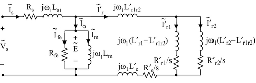
In the double-cage winding ω1L′r1r2 is the mutual reactance between cage r1 and cage r2. R′r1 and R′r2 are the resistances of cages r1 and r2, respectively. R′e and ω1L′e are the end-winding resistance and the end-winding leakage reactance of the end rings, respectively, if they are common to both cages. ω1L′r1 and ω1L′r2 are the leakage reactances of cages r1 and r2, respectively. The induced voltage is

With
one obtains alternatively

and

The resultant rotor impedance is now

In Eq. 3-62 the resulting rotor resistance R′r(s) and leakage inductance L′r(s) are slip (s) dependent. For an induction motor to be very efficient at rated slip the rotor resistance must be small. However, such a machine has a low starting torque. If the rotor resistance is relatively large the starting torque will be large, but the efficiency of such a machine will be very low. A double-squirrel cage solves this problem through a slip-dependent rotor resistance: at starting the currents mainly flow through the outer squirrel-cage winding having a large resistance, and at rated operation the currents flow mainly through the inner squirrel-cage winding having a small resistance. Triple- or quadruple-squirrel cage windings are employed for special applications only.
3.16 Summary
This chapter addresses first the normal operation of induction machines and the calculation of machine parameters, which are illustrated by flux plots. Power quality refers to the effects caused by induction machines due to their abnormal operation or by poorly designed machines. It discusses the influences of time and space harmonics on the rotating field, and the influence of current, voltage, and flux density harmonics on efficiency. This chapter highlights the detrimental effects of inter- and subharmonics on asynchronous and synchronous torque production, and the voltage stress induced by current source inverters and lightning surges. The applicability of harmonic models to three-phase induction machines is addressed. Static and dynamic rotor eccentricity, bearing currents, the operation of three-phase motors within a single-phase system, and the various classes and different equivalent circuits of induction machines are explained. Many application examples refer to the stable or unstable steady-state operation, the operation at under- or overvoltage and under- or over-frequency and combinations thereof. Calculation of asynchronous (integer, inter-, sub-) harmonic torques is performed in detail, whereas the generation of synchronous torque is mentioned. The calculation of the winding stress due to current and voltage-source inverters can be performed with either Mathematica or MATLAB.
3.17 Problems
Problem 3.1: Steady-State Stability
Figure P3.1a,b illustrates the torque–speed characteristics of a 10 kW three-phase induction motor with different rotor slot skewing with load torques TL1, TL2, and TL3. Comment on the steady-state stability of the equilibrium points A, B, C, D, E, F, G, H, I, and J in Fig. P3.1a and A, B, C, D, and E in Fig. P3.1b.

Problem 3.2: Phasor Diagram of Induction Machine at Fundamental Frequency and Steady-State Operation
Draw the phasor diagram for the equivalent circuit of Fig. P3.2. You may use the consumer reference system.

Problem 3.3: Analysis of an Induction Generator for a Wind-Power Plant
A Pout = 3.5 MW, VL-L = 2400 V, f = 60 Hz, p = 12 poles, nm-generator = 618 rpm, Y-connected squirrel-cage wind-power induction generator has the following parameters per phase referred to the stator: RS = 0.1 Ω, XS = 0.5 Ω, Xm → ∞ (that is, Xm can be ignored), R′r = 0.05 Ω, and X′r = 0.2 Ω. You may use the equivalent circuit of Fig. P3.2 with Xm and Rfe large so that they can be ignored. Calculate:
a) Synchronous speed nS in rpm.
b) Synchronous angular velocity ωS in rad/s.
c) Slip s.
d) Rotor current Ĩr′.
e) (Electrical) generating torque Tgen.
f) Slip sm where the maximum torque occurs.
g) Maximum torque Tmax in generation region.
Problem 3.4: E/f Control of a Squirrel-Cage Induction Motor [93]
The induction machine of Problem 3.3 is now used as a motor at nm-motor = 582 rpm. You may use the equivalent circuit of Fig. P3.2 with Xm and Rfe large so that they can be ignored. Calculate for E/f control:
b) Electrical torque Trated.
c) The frequency fnew at nm-new = 300 rpm, and Trated.
d) The new slip snew.
Problem 3.5: V/f Control of a Squirrel-Cage Induction Motor [93]
The induction machine of Problem 3.3 is now used as a motor at nm-motor = 582 rpm. You may use the equivalent circuit of Fig. P3.2 with Xm and Rfe large so that they can be ignored. Calculate for V/f control:
b) The new slip snew.
c) The frequency fnew at nm-new = 300 rpm, and Trated.
Problem 3.6: Steady-State Operation at Undervoltage
A Pout = 100 hp, VL-L_rat = 480 V, f = 60 Hz, p = 6 pole three-phase induction motor runs at full load and rated voltage with a slip of 3%. Under conditions of stress on the power supply system, the line-to-line voltage drops to VL-L_low = 450 V. If the load is of the constant torque type, compute for the lower voltage:
a) The slip slow (use small-slip approximation).
b) The shaft speed nm_low in rpm.
c) The output power Pout_low.
d) The rotor copper loss Pcur_low = Ir′2Rr′ in terms of the rated rotor copper loss at rated voltage.
Problem 3.7: Steady-State Operation at Overvoltage
Repeat Problem 3.6 for the condition when the line-to-line voltage of the power supply system increases to VL-L_high = 500 V.
Problem 3.8: Steady-State Operation at Undervoltage and Under-Frequency
A Pout_rat = 100 hp, VL-L_rat = 480 V, f = 60 Hz, p = 6 pole three-phase induction motor runs at full load and rated voltage and frequency with a slip of 3%. Under conditions of stress on the power supply system the terminal voltage and the frequency drop to VL-L_low = 450 V and flow = 59.5 Hz, respectively. If the load is of the constant torque type, compute for the lower voltage and frequency:
a) The slip (use small-slip approximation).
b) The shaft speed in rpm.
c) The hp output.
d) The rotor copper loss Pcur_low = Ir′2Rr′ in terms of the rated rotor copper loss at rated frequency and voltage.
Problem 3.9: Steady-State Operation at Overvoltage and Over-Frequency
A Pout_rat = 100 hp, VL-L_rat = 480 V, f = 60 Hz, p = 6 pole three-phase induction motor runs at full load and rated voltage and frequency with a slip of 3%. Assume the terminal voltage and the frequency increase to VL-L_high = 500 V and fhigh = 60.5 Hz, respectively. If the load is of the constant torque type, compute for the lower voltage and frequency:
a) The slip (use small-slip approximation).
b) The shaft speed in rpm.
c) The hp output.
d) The rotor copper loss Pcur_ high = Ir′2Rr′ in terms of the rated rotor copper loss at rated frequency and voltage.
Problem 3.10: Calculation of the Maximum Critical Speeds nmcriticalmotoring and nmcriticalregeneration for Motoring and Regeneration, Respectively [93]
A VL-L_rat = 480 V, frat = 60 Hz, nmrat = 1760 rpm, 4-pole, Y-connected squirrel-cage induction machine has the following parameters per phase referred to the stator: RS = 0.2 Ω, XS = 0.5 Ω, Xm = 20 Ω, R′r = 0.1 Ω, X′r = 0.8 Ω. Use the equivalent circuit of Fig. P3.10.1.

A hybrid car employs the induction machine with the above-mentioned parameters for the electrical part of the drive.
a) Are the characteristics of Figure P3.10.2 (for a = f/frated< 1) either E/f control or V/f control?

b) Compute the rated electrical torque Trat , the rated angular velocity ωmrat and the rated output power Prat (see operating point Q1 of Figure P3.10.2).
c) Calculate the maximum critical motoring speed nmcriticalmotoring, whereby rated output power (Prat = Trat · ωmrat) is delivered by the machine at the shaft (see operating point Q2 of Fig. P3.10.2).
d) Calculate the maximum critical speed nmcriticalregeneration, whereby rated power is absorbed at the shaft by the machine (see operating point Q3 of Fig. P3.10.2).
e) In order to increase the critical motoring speed to about 3 times the rated speed nmrat an engineer proposes to decrease Xs and X′r by a factor of two. Will this accomplish the desired speed increase? Note that the resistances Rs and R′r are so small that no significant speed increase can be expected by changing them.
Problem 3.11: Torque Characteristic of Induction Machine with Fundamental and Subharmonic Fields
The equivalent circuit of a voltage-source-fed induction motor is shown in Fig. 3.38. The fundamental angular frequency of the voltage source is ω1 and the time-harmonic angular frequency is hω1 (caused by imperfections of the voltage-source inverter).
The parameters of the three-phase induction motor are as follows: VL-L = 460 V, Y-connected, p = 2 poles, nrated = 3528 rpm, f = 60 Hz, Rs = 1 Ω, ω1Lsℓ = 2 Ω, ω1Lm = ∞ (you may neglect the magnetizing branch), R′r = 1 Ω, ω1L′rℓ = 2 Ω.
a) Compute a few points (e.g., Te1(s1 = 0), Te1(s1 = s1max +), Te1(s1 = s1max–),Te1(s1 = 1.0)) and sketch the fundamental torque characteristic Te1 = f(s1) in Nm, where s1 is the slip of the rotor with respect to the fundamental positively rotating (forward rotating, positive sequence) field.
b) Provided a negatively rotating (backward rotating, negative sequence) voltage time subharmonic of 30 Hz (h = 0.5) is present with a magnitude of Vs0.5/Vs1 = 0.10 compute a few points (e.g., Te0.5(s0.5 = 0), Te0.5(s0.5 = s0.5max +), Te0.5(s0.5 = s0.5max–), Te0.5(s0.5 = 1.0)) of this subharmonic torque characteristic Te0.5 = f(s0.5) in Nm.
c) Sketch the subharmonic torque characteristic Te0.5 = f(s0.5) in Nm.
d) Sketch the total torque characteristics (Te1 + Te0.5) = f(s1) in Nm.
e) What is the starting torque (at s1 = 1) without and with this (h = 0.5) time subharmonic?
Problem 3.12: Voltage Stress due to Current Ripples in Stator Windings of an Induction Motor Fed by a Current-Source Inverter Through a Cable of 10 m Length
Current ripples due to PWM current-source inverters cause voltage stress in windings of machines. The configuration of Fig. E3.14.1 represents the first two turns of the winding of an induction motor. Each turn can be represented by four segments having an inductance Li, a resistance Ri, a capacitance to ground (frame) Ci, and some interturn capacitances Cij and inductances Lij. Figure E.3.14.2 represents a detailed equivalent circuit for the configuration of Fig. E3.14.1. To simplify the analysis neglect the capacitances Cij and the inductances Lij. This leads to the circuit in Fig. E3.14.3, where the winding is fed by a PWM current source. One obtains the 15 differential equations as listed below.


The parameters are
R1 = R2 = R3 = R4 = R5 = R6 = R7 = R8 = 25 μΩ;
L1 = L3 = L5 = L7 = 1 mH, and
L2 = L4 = L6 = L8 = 10 mH; C1 = 0.2 μF for the cable of 10 m length; C3 = C5 = C7 = 0.7 pF,
C2 = C4 = C6 = C8 = 7 pF, C15 = C37 = 0.35 pF,
C26 = C48 = 3.5 pF; G1 = G3 = G5 = G7 = 1/(5000 Ω),
G2 = G4 = G6 = G8 = 1/(500 Ω); and
L15 = L37 = 0.005 mH, L26 = L48 = 0.01 mH.
Z is either 1 μΩ (short-circuit) or 1 MΩ (open-circuit).
Assume a PWM triangular current-step function is(t) as indicated in Fig. E3.14.4. Using Mathematica or MATLAB compute all state variables for the time period from t = tcalculate = 0 to 2.1 ms. Plot the voltages (v1 – v5), (v2 – v6), (v3 – v7), and (v4 – v8) for t = tplot = 2 ms. Note that the computing time t = tcalculate = 2.1 ms must be larger than the plotting time t = tplot = 2 ms.
Problem 3.13: Voltage Stress within the Stator Winding of a Large Induction Hydrogenerator Due to Lightning Surge
Lightning surges cause voltage stress in windings of machines. The configuration of Fig. E3.14.1 represents the first two turns of the winding of an induction generator operating without transformer on the 2400 VL-L power system. Each turn can be represented by four segments having an inductance Li, a resistance Ri, a capacitance to ground (frame) Ci, and some interturn capacitances Cij and inductances Lij. Figure E.3.14.2 represents a detailed equivalent circuit for the configuration of Fig. E3.14.1. To simplify the analysis neglect the capacitances Cij and the inductances Lij. This leads to the circuit Fig. E3.14.3. One obtains the 15 differential equations as listed in Problem 3.12.
The parameters are
R1 = R2 = R3 = R4 = R5 = R6 = R7 = R8 = 25 μΩ;
L1 = L3 = L5 = L7 = 1 mH, and
L2 = L4 = L6 = L8 = 10 mH; C1 = C3 = C5 = C7 = 7 pF,
C2 = C4 = C6 = C8 = 70 pF, C15 = C37 = 3.5 pF,
C26 = C48 = 35 pF; G1 = G3 = G5 = G7 = 1/(5000 Ω),
G2 = G4 = G6 = G8 = 1/(500 Ω); and
L15 = L37 = 0.005 mH, L26 = L48 = 0.01 mH.
Z is either 1 μΩ (short-circuit) or 1 MΩ (open-circuit), Isurge = 10,000 A.
Assume a lightning surge function is(t) as indicated in Fig. P3.13. Using Mathematica or MATLAB compute all state variables for the time period from t = tcalculate = 0 to 2.1 ms. Plot the voltages (v1 – v5), (v2 – v6), (v3 – v7), and (v4 – v8) for t = tplot = 2 ms. Note that the computing time t = tcalculate = 2.1 ms must be larger than the plotting time t = tplot = 2 ms.

Problem 3.14: Harmonics of Current and Voltage Wave Shapes
Determine the Fourier coefficients of the currents and voltages of Figs. 3.33, 3.34, and E3.6.7a,b. Show that for a given sampling rate the Nyquist criterion is satisfied which in turn means that the approximation error of the reconstructed function is minimum.