
Chapter 21. Time Series and Autocorrelation
A big part of statistics, particularly for financial and econometric data, is analyzing time series, data that are autocorrelated over time. That is, one observation depends on previous observations and the order matters. Special care needs to be taken to account for this dependency. R has a number of built-in functions and packages to make working with time series easier.
21.1. Autoregressive Moving Average
One of the most common ways of fitting time series models is to use autoregressive (AR), moving average (MA) or both (ARMA). These models are well represented in R and are fairly easy to work with. The formula for an ARMA(p, q) is
where
is white noise, which is essentially random data.
AR models can be thought of as linear regressions of the current value of the time series against previous values. MA models are, similarly, linear regressions of the current value of the time series against current and previous residuals.
For an illustration, we will make use of the World Bank API to download gross domestic product (GDP) for a number of countries from 1960 through 2011.
> # load the World Bank API package
> require(WDI)
> # pull the data
> gdp <- WDI(country=c("US", "CA", "GB", "DE", "CN", "JP", "SG", "IL"),
+ indicator=c("NY.GDP.PCAP.CD", "NY.GDP.MKTP.CD"),
+ start=1960, end=2011)
> # give it good names
> names(gdp) <- c("iso2c", "Country", "Year", "PerCapGDP", "GDP")
After downloading, we can inspect the data, which are stored in long country-year format with a plot of per capita GDP shown in Figure 21.1a. Figure 21.1b shows absolute GDP, illustrating that while China’s GDP has jumped significantly in the past ten years, its per capita GDP has only marginally increased.

> head(gdp)
iso2c Country Year PerCapGDP GDP
1 CA Canada 1960 2294.569 41093453545
2 CA Canada 1961 2231.294 40767969454
3 CA Canada 1962 2255.230 41978852041
4 CA Canada 1963 2354.839 44657169109
5 CA Canada 1964 2529.518 48882938810
6 CA Canada 1965 2739.586 53909570342
> require(ggplot2)
> require(scales)
> # per capita GDP
> ggplot(gdp, aes(Year, PerCapGDP, color=Country, linetype=Country)) +
+ geom line() + scale y continuous(label=dollar)
>
> require(useful)
> # absolute GDP
> ggplot(gdp, aes(Year, GDP, color=Country, linetype=Country)) +
+ geom line() +
+ scale y continuous(label=multiple format(extra=dollar,
+ multiple="M"))
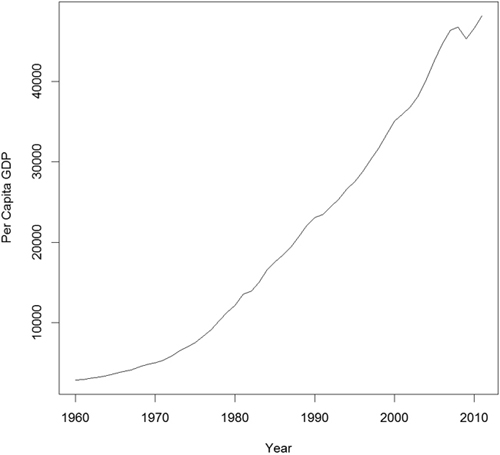
First we will only look at only one time series, so we extract the data for the United States. See Figure 21.2.
> # get US data
> us <- gdp$PerCapGDP[gdp$Country == "United States"]
> # convert it to a time series
> us <- ts(us, start = min(gdp$Year), end = max(gdp$Year))
> us
Time Series:
Start = 1960
End = 2011
Frequency = 1
[1] 2881.100 2934.553 3107.937 3232.208 3423.396 3664.802
[7] 3972.123 4152.020 4491.424 4802.642 4997.757 5360.178
[13] 5836.224 6461.736 6948.198 7516.680 8297.292 9142.795
[19] 10225.307 11301.682 12179.558 13526.187 13932.678 15000.086
[25] 16539.383 17588.810 18427.288 19393.782 20703.152 22039.227
[31] 23037.941 23443.263 24411.143 25326.736 26577.761 27559.167
[37] 28772.356 30281.636 31687.052 33332.139 35081.923 35912.333
[43] 36819.445 38224.739 40292.304 42516.393 44622.642 46349.115
[49] 46759.560 45305.052 46611.975 48111.967
> plot(us, ylab = "Per Capita GDP", xlab = "Year")
Another way to assess a time series is to view its autocovariance function (ACF) and partial autocovariance function (PACF). In R this is done with the appropriately named acf and pacf functions.
The ACF shows the correlation of a time series with lags of itself. That is, how much the time series is correlated with itself at one lag, at two lags, at three lags and so on.
The PACF is a little more complicated. The autocorrelation at lag one can have lingering effects on the autocorrelation at lag two and onward. The partial autocorrelation is the amount of correlation between a time series and lags of itself that is not explained by a previous lag. So, the partial autocorrelation at lag two is the correlation between the time series and its second lag that is not explained by the first lag.
The ACF and PACF for the U.S. Per Capita GDP data are shown in Figure 21.3. Vertical lines that extend beyond the horizontal line indicate autocorrelations and partial autocorrelations that are significant at those lags.
> acf(us)
> pacf(us)
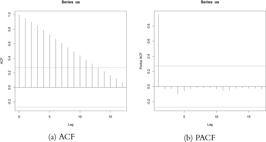
Figure 21.3 ACF and PACF of U.S. Per Capita GDP. These plots are indicative of a time series that is not stationary.
This time series needs a number of transformations before it can be properly modeled. Its upward trend shows that it is not stationary1 (the data are in current U.S. dollars, so inflation is not the cause). That can be fixed by diffing the series or applying some other transformation. Diffing is the process of subtracting one observation from another and can be done on any number of observations. For instance, we start with a series
1. Being stationary requires that the mean and variance of a time series are constant for the whole series.
x = [ 1 4 8 2 6 6 5 3 ]. Diffing it yields x(1) = [ 3 4 –6 4 0 –1 –2 ], which is the difference between successive elements. Diffing twice iteratively diffs the diffs, so x(2) = [ 1 –10 10 –4 –1 –1 ]. Observe that for each level of diffing, there is one fewer element in the series. Doing this in R involves the diff function. The differences argument controls how many diffs are iteratively calculated. The lag determines which elements get subtracted from each other. A lag of 1 subtracts successive elements, while a lag of 2 subtracts elements that are two indices away from each other.
> x <- c(1, 4, 8, 2, 6, 6, 5, 3)
> # one diff
> diff(x, differences = 1)
[1] 3 4 -6 4 0 -1 -2
> # two iterative diffs
> diff(x, differences = 2)
[1] 1 -10 10 -4 -1 -1
> # equivalent to one diff
> diff(x, lag = 1)
[1] 3 4 -6 4 0 -1 -2
> # diff elements that are two indices apart
> diff(x, lag = 2)
[1] 7 -2 -2 4 -1 -3
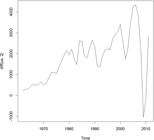
Figuring out the correct number of diffs can be a tiresome process. Fortunately, the forecast package has a number of functions to make working with time series data easier, including determining the optimal number of diffs. The result is shown in Figure 21.4.
> require(forecast)
> ndiffs(x = us)
[1] 2
> plot(diff(us, 2))
While R offers individual ar and ma functions, a better option is the arima function, which can fit both AR and MA models and the combined ARMA model. It is even more robust in that it can diff the series and fit seasonal effects. Traditionally, the right order of each component of the model is determined by analyzing the ACF and PACF. This can be highly subjective, so fortunately forecast contains auto.arima, which will figure out the best specification.
> usBest <- auto.arima(x = us)
> usBest
Series: us
ARIMA(2,2,1)
Coefficients:
ar1 ar2 ma1
0.4181 -0.2567 -0.8102
s.e. 0.1632 0.1486 0.1111
sigma^2 estimated as 269726: log likelihood=-384.05
AIC=776.1 AICc=776.99 BIC=783.75
The function determined that an ARMA(2,1) (an AR(2) component and an MA(1) component) with two diffs is the optimal model based on minimum AICC (that is, AIC that is “corrected” to give a greater penalty to model complexity). The two diffs actually make this an ARIMA model rather than an ARMA model where the I stands for integrated. If this model is a good fit, then the residuals should resemble white noise. Figure 21.5 shows the ACF and PACF of the residuals for the ideal model. They resemble the pattern for white noise, confirming our model selection.
> acf(usBest$residuals)
> pacf(usBest$residuals)

The coefficients for an ARIMA model are the AR and MA components.
> coef(usBest)
ar1 ar2 ma1
0.4181109 -0.2567494 -0.8102419
Making predictions based on an ARIMA model is much the same as with any other model type, using the predict function.
> # predict 5 years into the future and include the standard error
> predict(usBest, n.ahead = 5, se.fit = TRUE)
$pred
Time Series:
Start = 2012
End = 2016
Frequency = 1
[1] 49292.41 50289.69 51292.41 52344.45 53415.70
$se
Time Series:
Start = 2012
End = 2016
Frequency = 1
[1] 519.3512 983.3778 1355.0380 1678.3930 2000.3464
Visualizing this is easy enough but using the forecast function makes it even easier, as seen in Figure 21.6.
> # make a prediction for 5 years out
> theForecast <- forecast(object = usBest, h = 5)
> # plot it
> plot(theForecast)

Figure 21.6 Five year prediction of U.S. GDP. The think line is the point estimate and the shaded regions represent the confidence intervals.
21.2. VAR
When dealing with multiple time series where each depends on its own past, others’ pasts and others’ presents, things get more complicated. The first thing we will do is convert all of the GDP data into a multivariate time series. To do this we first cast the data.frame to wide format then call ts to convert it. The result is shown in Figure 21.7.
> # load reshape2
> require(reshape2)
> # cast the data.frame to wide format
> gdpCast <- dcast(Year ~ Country,
+ data=gdp[, c("Country", "Year", "PerCapGDP")],
+ value.var="PerCapGDP")
> head(gdpCast)
Year Canada China Germany Israel Japan Singapore
1 1960 2294.569 92.01123 NA 1365.683 478.9953 394.6489
2 1961 2231.294 75.87257 NA 1595.860 563.5868 437.9432
3 1962 2255.230 69.78987 NA 1132.383 633.6403 429.5377
4 1963 2354.839 73.68877 NA 1257.743 717.8669 472.1830
5 1964 2529.518 83.93044 NA 1375.943 835.6573 464.3773
6 1965 2739.586 97.47010 NA 1429.319 919.7767 516.2622
United Kingdom United States
1 1380.306 2881.100
2 1452.545 2934.553
3 1513.651 3107.937
4 1592.614 3232.208
5 1729.400 3423.396
6 1850.955 3664.802
> # remove first 10 rows since Germany did not have
>
> # convert to time series
> gdpTS <- ts(data=gdpCast[, -1], start=min(gdpCast$Year),
+ end=max(gdpCast$Year))
>
> # build a plot and legend using base graphics
> plot(gdpTS, plot.type="single", col=1:8)
> legend("topleft", legend=colnames(gdpTS), ncol=2, lty=1,
+ col=1:8, cex=.9)
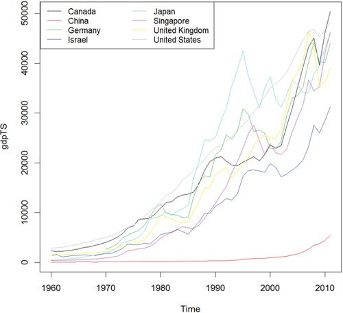
Figure 21.7 Time series plot of GDP data for all countries in the data. This is the same information as in Figure 21.1a, but this was built using base graphics.
Before proceeding we have to deal with the NAs for Germany. For some reason the World Bank does not have data on Germany’s GDP before 1970. There are other resources, such as the St. Louis Federal Reserve Economic Data (FRED), but their data do not agree well with the World Bank data, so we remove Germany from our data.
> gdpTS <- gdpTS[, which(colnames(gdpTS) != "Germany")]
The most common way of fitting a model to multiple time series is to use a vector autoregressive (VAR) model. The equation for a VAR is
is white noise.
While ar can compute a VAR, it often has problems with singular matrices when the AR order is high, so it is better to use VAR from the vars package. To check whether the data should be diffed, we use the ndiffs function on gdpTS and then apply that number of diffs. The diffed data are shown in Figure 21.8, which exhibits greater stationarity than Figure 21.7.
> numDiffs <- ndiffs(gdpTS)
> numDiffs
[1] 1
> gdpDiffed <- diff(gdpTS, differences=numDiffs)
> plot(gdpDiffed, plot.type="single", col=1:7)
> legend("bottomleft", legend=colnames(gdpDiffed), ncol=2, lty=1,
+ col=1:7, cex=.9)

Now that the data are prepared, we can fit a VAR using VAR. This essentially fits a separate regression using lm of each time series on the lags of itself and the other series. This is evidenced in the coefficient plot for the Canada and Japan models, shown in Figure 21.9.
> require(vars)
> # fit the model
> gdpVar <- VAR(gdpDiffed, lag.max = 12)
> # chosen order
> gdpVar$p
AIC(n)
6
>
> # names of each of the models
> names(gdpVar$varresult)
[1] "Canada" "China" "Israel"
[4] "Japan" "Singapore" "United.Kingdom"
[7] "United.States"
>
> # each model is actually an lm object
> class(gdpVar$varresult$Canada)
[1] "lm"
> class(gdpVar$varresult$Japan)
[1] "lm"
>
> # each model has its own coefficients
> head(coef(gdpVar$varresult$Canada))
Canada.l1 China.l1 Israel.l1
-1.07854513 -7.28241774 1.06538174
Japan.l1 Singapore.l1 United.Kingdom.l1
-0.45533608 -0.03827402 0.60149182
> head(coef(gdpVar$varresult$Japan))
Canada.l1 China.l1 Israel.l1
1.8045012 -19.7904918 -0.1507690
Japan.l1 Singapore.l1 United.Kingdom.l1
1.3344763 1.5738029 0.5707742
>
> require(coefplot)
> coefplot(gdpVar$varresult$Canada)
> coefplot(gdpVar$varresult$Japan)

Predictions for this model are done just like with any other model, using the predict function.
> predict(gdpVar, n.ahead = 5)
$Canada
fcst lower upper CI
[1,] -12459.46 -13284.63 -11634.30 825.1656
[2,] 15067.05 14106.02 16028.08 961.0344
[3,] 20632.99 19176.30 22089.69 1456.6943
[4,] -103830.42 -105902.11 -101758.73 2071.6904
[5,] 124483.19 119267.39 129699.00 5215.8046
$China
fcst lower upper CI
[1,] -470.5917 -523.6101 -417.5733 53.01843
[2,] 899.5380 826.2362 972.8399 73.30188
[3,] 1730.8087 1596.4256 1865.1918 134.38308
[4,] -3361.7713 -3530.6042 -3192.9384 168.83288
[5,] 2742.1265 2518.9867 2965.2662 223.13974
$Israel
fcst lower upper CI
[1,] -6686.711 -7817.289 -5556.133 1130.578
[2,] -39569.216 -40879.912 -38258.520 1310.696
[3,] 62192.139 60146.978 64237.300 2045.161
[4,] -96325.105 -101259.427 -91390.783 4934.322
[5,] -12922.005 -24003.839 -1840.171 11081.834
$Japan
fcst lower upper CI
[1,] -14590.8574 -15826.761 -13354.954 1235.903
[2,] -52051.5807 -53900.387 -50202.775 1848.806
[3,] -248.4379 -3247.875 2750.999 2999.437
[4,] -51465.6686 -55434.880 -47496.457 3969.212
[5,] -111005.8032 -118885.682 -103125.924 7879.879
$Singapore
fcst lower upper CI
[1,] -35923.80 -36071.93 -35775.67 148.1312
[2,] 54502.69 53055.85 55949.53 1446.8376
[3,] -43551.08 -47987.48 -39114.68 4436.3991
[4,] -99075.95 -107789.86 -90362.04 8713.9078
[5,] 145133.22 135155.64 155110.81 9977.5872
$United.Kingdom
fcst lower upper CI
[1,] -19224.96 -20259.35 -18190.56 1034.396
[2,] 31194.77 30136.87 32252.67 1057.903
[3,] 27813.08 24593.47 31032.68 3219.604
[4,] -66506.90 -70690.12 -62323.67 4183.226
[5,] 93857.98 88550.03 99165.94 5307.958
$United.States
fcst lower upper CI
[1,] -657.2679 -1033.322 -281.2137 376.0542
[2,] 11088.0517 10614.924 11561.1792 473.1275
[3,] 2340.6277 1426.120 3255.1350 914.5074
[4,] -5790.0143 -7013.843 -4566.1855 1223.8288
[5,] 24306.5309 23013.525 25599.5373 1293.0064
21.3. GARCH
A problem with ARMA models is that they do not handle extreme events or high volatility well. To overcome this a good tool to use is generalized autoregressive conditional heteroskedasticity or the GARCH family of models, which in addition to modeling the mean of the process also model the variance.
The model for the variance in a GARCH(m, s) is
and
is generalized white noise.
For this example we download AT&T ticker data using the quantmod package.
> require(quantmod)
> att <- getSymbols("T", auto.assign = FALSE)
This loads the data into an xts object from the xts package, which is a more robust time series object that, among many other improvements, can handle irregularly spaced events. These objects even have improved plotting over ts, as seen in Figure 21.10.

> require(xts)
> # show data
> head(att)
T.Open T.High T.Low T.Close T.Volume T.Adjusted
2007-01-03 35.67 35.78 34.78 34.95 33694300 25.06
2007-01-04 34.95 35.24 34.07 34.50 44285400 24.74
2007-01-05 34.40 34.54 33.95 33.96 36561800 24.35
2007-01-08 33.40 34.01 33.21 33.81 40237400 24.50
2007-01-09 33.85 34.41 33.66 33.94 40082600 24.59
2007-01-10 34.20 35.00 31.94 34.03 29964300 24.66
> plot(att)
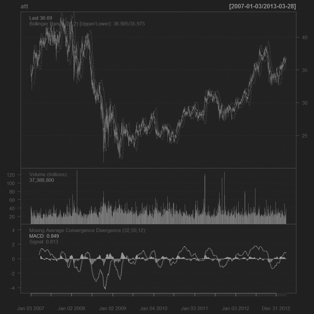
For those used to financial terminal charts, the chartSeries function should be comforting. It created the chart shown in Figure 21.11.
> chartSeries(att)
> addBBands()
> addMACD(32, 50, 12)
We are only interested in the closing price, so we create a variable holding just that.
> attClose <- att$T.Close
> class(attClose)
[1] "xts" "zoo"
> head(attClose)
T.Close
2007-01-03 34.95
2007-01-04 34.50
2007-01-05 33.96
2007-01-08 33.81
2007-01-09 33.94
2007-01-10 34.03
The package most widely considered to be the best for fitting GARCH models is rugarch. There are other packages for fitting GARCH models, such as tseries, fGarch and bayesGARCH, but we will focus on rugarch.
Generally, a GARCH(1,1) will be sufficient so we will fit that model to the data. The first step is setting up the model specification using ugarchspec. We specify the volatility to be modeled as a GARCH(1, 1) and the mean to be modeled as an ARMA(1, 1). We also specify that the innovation distribution should be the t distribution.
> require(rugarch)
> attSpec <- ugarchspec(variance.model=list(model="sGARCH",
+ garchOrder=c(1, 1)),
+ mean.model=list(armaOrder=c(1, 1)),
+ distribution.model="std")
The next step is to fit the model using ugarchfit.
> attGarch <- ugarchfit(spec = attSpec, data = attClose)
Printing the model spits out a lot of information, including the coefficients, standard errors, AIC and BIC. Most of this, such as the statistics on residuals, tests, AIC and BIC are diagnostic measures on the quality of the fit. The optimal parameters, seen near the top, are the crux of the model.
> attGarch
*---------------------------------*
* GARCH Model Fit *
*---------------------------------*
Conditional Variance Dynamics
-----------------------------------
GARCH Model : sGARCH(1,1)
Mean Model : ARFIMA(1,0,1)
Distribution : std
Optimal Parameters
------------------------------------
Estimate Std. Error t value Pr(>|t|)
mu 35.159848 1.328210 26.47160 0.000000
ar1 0.997009 0.001302 765.82269 0.000000
ma1 -0.009937 0.026801 -0.37078 0.710800
omega 0.001335 0.000692 1.92969 0.053645
alpha1 0.069952 0.014968 4.67328 0.000003
beta1 0.925012 0.015400 60.06615 0.000000
shape 7.581676 1.404834 5.39685 0.000000
Robust Standard Errors:
Estimate Std. Error t value Pr(>|t|)
mu 35.159848 0.541745 64.9011 0.000000
ar1 0.997009 0.001155 862.8530 0.000000
ma1 -0.009937 0.028813 -0.3449 0.730171
omega 0.001335 0.000795 1.6781 0.093319
alpha1 0.069952 0.018096 3.8657 0.000111
beta1 0.925012 0.018992 48.7047 0.000000
shape 7.581676 1.332371 5.6904 0.000000
LogLikelihood : -776.0355
Information Criteria
------------------------------------
Akaike 0.99750
Bayes 1.02139
Shibata 0.99746
Hannan-Quinn 1.00638
Q-Statistics on Standardized Residuals
------------------------------------
statistic p-value
Lag[1] 0.5528 0.4572
Lag[p+q+1][3] 3.2738 0.0704
Lag[p+q+5][7] 6.8829 0.2295
d.o.f=2
H0 : No serial correlation
Q-Statistics on Standardized Squared Residuals
------------------------------------
statistic p-value
Lag[1] 0.005088 0.94314
Lag[p+q+1][3] 3.989786 0.04578
Lag[p+q+5][7] 5.817106 0.32442
d.o.f=2
ARCH LM Tests
------------------------------------
Statistic DoF P-Value
ARCH Lag[2] 2.229 2 0.3281
ARCH Lag[5] 4.597 5 0.4670
ARCH Lag[10] 9.457 10 0.4893
Nyblom stability test
------------------------------------
Joint Statistic: 1.5032
Individual Statistics:
mu 0.18923
ar1 0.09786
ma1 0.24465
omega 0.13823
alpha1 0.62782
beta1 0.52974
shape 0.47109
Asymptotic Critical Values (10% 5% 1%)
Joint Statistic: 1.69 1.9 2.35
Individual Statistic: 0.35 0.47 0.75
Sign Bias Test
------------------------------------
t-value prob sig
Sign Bias 0.8259 0.4090
Negative Sign Bias 0.8228 0.4108
Positive Sign Bias 0.3965 0.6918
Joint Effect 3.0136 0.3895
Adjusted Pearson Goodness-of-Fit Test:
------------------------------------
group statistic p-value(g-1)
1 20 28339 0
2 30 44012 0
3 40 59699 0
4 50 75391 0
Elapsed time : 0.8640492
Figure 21.12 shows a time series plot and the ACF of the residuals from the model.
> # attGarch is an S4 object so its slots are accessed by @
> # the slot fit is a list, so its elements are accessed as usual with $
> plot(attGarch@fit$residuals, type="l")
> plot(attGarch, which=10)

To judge the quality of this model, we build a few models with different mean specifications—all GARCH(1, 1)—and compare their AICs.
> # ARMA(1,1)
> attSpec1 <- ugarchspec(variance.model=list(model="sGARCH",
+ garchOrder=c(1, 1)),
+ mean.model=list(armaOrder=c(1, 1)),
+ distribution.model="std")
> # ARMA(0,0)
> attSpec2 <- ugarchspec(variance.model=list(model="sGARCH",
+ garchOrder=c(1, 1)),
+ mean.model=list(armaOrder=c(0, 0)),
+ distribution.model="std")
> # ARMA(0,2)
> attSpec3 <- ugarchspec(variance.model=list(model="sGARCH",
+ garchOrder=c(1, 1)),
+ mean.model=list(armaOrder=c(0, 2)),
+ distribution.model="std")
> # ARMA(1,2)
> attSpec4 <- ugarchspec(variance.model=list(model="sGARCH",
+ garchOrder=c(1, 1)),
+ mean.model=list(armaOrder=c(1, 2)),
+ distribution.model="std")
>
> attGarch1 <- ugarchfit(spec=attSpec1, data=attClose)
> attGarch2 <- ugarchfit(spec=attSpec2, data=attClose)
> attGarch3 <- ugarchfit(spec=attSpec3, data=attClose)
> attGarch4 <- ugarchfit(spec=attSpec4, data=attClose)
>
> infocriteria(attGarch1)
Akaike 0.9974974
Bayes 1.0213903
Shibata 0.9974579
Hannan-Quinn 1.0063781
> infocriteria(attGarch2)
Akaike 5.108533
Bayes 5.125600
Shibata 5.108513
Hannan-Quinn 5.114877
> infocriteria(attGarch3)
Akaike 3.406478
Bayes 3.430371
Shibata 3.406438
Hannan-Quinn 3.415359
> infocriteria(attGarch4)
Akaike 0.9963163
Bayes 1.0236224
Shibata 0.9962647
Hannan-Quinn 1.0064656
This shows that the first and fourth models were the best, according to AIC and BIC and the other criteria.
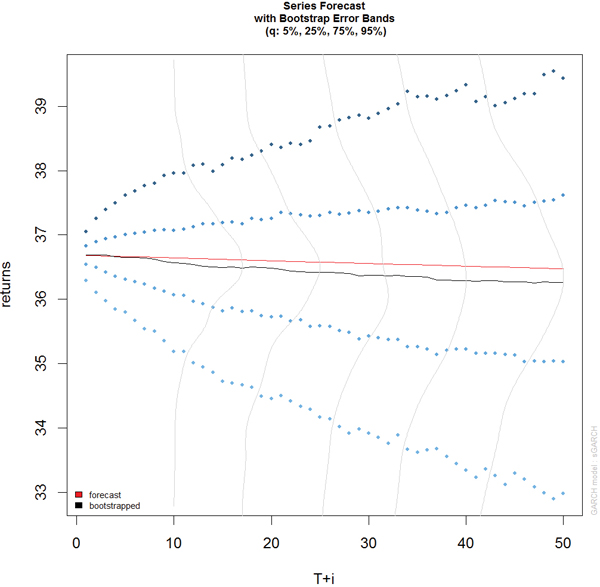
Predicting with objects from rugarch is done through the ugarchboot function, which can then be plotted as seen in Figure 21.13.
> attPred <- ugarchboot(attGarch, n.ahead=50,
+ method = c("Partial", "Full")[1])
> plot(attPred, which=2)
Because this is stock data, it is worth computing the model on the log returns instead of the actual closing prices.
> # diff the logs, drop the first one which is now NA
> attLog <- diff(log(attClose))[-1]
> # build the specification
> attLogSpec <- ugarchspec(variance.model=list(model="sGARCH",
+ garchOrder=c(1, 1)),
+ mean.model=list(armaOrder=c(1, 1)),
+ distribution.model="std")
> # fit the model
> attLogGarch <- ugarchfit(spec=attLogSpec, data=attLog)
> infocriteria(attLogGarch)
Akaike -5.870043
Bayes -5.846138
Shibata -5.870083
Hannan-Quinn -5.861158
This led to a significant drop in AIC.
It is important to remember that the purpose of GARCH models is not to fit the signal better but to capture the volatility better.
21.4. Conclusion
Time series play a crucial role in many fields, particularly finance and some physical sciences. The basic building block in R for time series is the ts object, which has been greatly extended by the xts object. The most common types of models are ARMA, VAR and GARCH, which are fitted by the arima, VAR and ugarchfit functions, respectively.