
Chapter 16. Linear Models
The workhorse of statistical analysis is the linear model, particularly regression. Originally invented by Francis Galton to study the relationships between parents and children, which he described as regressing to the mean, it has become one of the most widely used modeling techniques and has spawned other models such as generalized linear models, regression trees, penalized regression and many others. In this chapter we focus on simple and multiple regression and some basic generalized linear models.
16.1. Simple Linear Regression
In its simplest form regression is used to determine the relationship between two variables. That is, given one variable, it tells us what we can expect from the other variable. This powerful tool, which is frequently taught and can accomplish a great deal of analysis with minimal effort, is called simple linear regression.
Before we go any further, we clarify some terminology. The outcome variable (what we are trying to predict) is called the response, and the input variable (what we are using to predict) is the predictor. Fields outside of statistics use other terms, such as measured variable, outcome variable and experimental variable for response, and covariate, feature and explanatory variable for predictor. Worst of all are the terms dependent (response) and independent (predictor) variables. These very names are misnomers. According to probability theory, if variable y is dependent on variable x then variable x cannot be independent of variable y. So we stick with the terms response and predictor exclusively.
The general idea behind simple linear regression is using the predictor to come up with some average value of the response. The relationship is defined as
where
which is to say that there are normally distributed errors.
Equation 16.1 is essentially describing a straight line that goes through the data where a is the y-intercept and b is the slope. This is illustrated using fathers’ and sons’ height data, which are plotted in Figure 16.1. In this case we are using the fathers’ heights as the predictor and the sons’ heights as the response. The blue line running through the points is the regression line and the grey band around it represents the uncertainty in the fit.
> require(UsingR)
> require(ggplot2)
> head(father.son)
fheight sheight
1 65.04851 59.77827
2 63.25094 63.21404
3 64.95532 63.34242
4 65.75250 62.79238
5 61.13723 64.28113
6 63.02254 64.24221
> ggplot(father.son, aes(x=fheight, y=sheight)) + geom_point() +
+ geom_smooth(method="lm") + labs(x="Fathers", y="Sons")
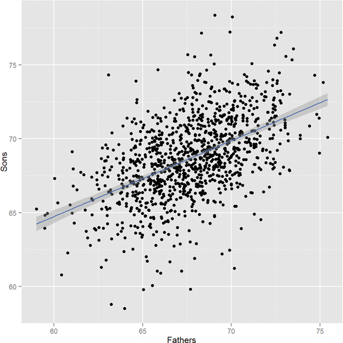
Figure 16.1 Using fathers’ heights to predict sons’ heights using simple linear regression. The fathers’ heights are the predictors and the sons’ heights are the responses. The blue line running through the points is the regression line and the grey band around it represents the uncertainty in the fit.
While that code generated a nice graph showing the results of the regression (generated with geom smooth(method="lm")), it did not actually make those results available to us. To actually calculate a regression use the lm function.
> heightsLM <- lm(sheight ~ fheight, data = father.son)
> heightsLM
Call:
lm(formula = sheight ~ fheight, data = father.son)
Coefficients:
(Intercept) fheight
33.8866 0.5141
Here we once again see the formula notation that specifies to regress sheight (the response) on fheight (the predictor), using the father.son data, and adds the intercept term automatically. The results show coefficients for (Intercept) and fheight which is the slope for the fheight, predictor. The interpretation of this is that, for every extra inch of height in a father, we expect an extra half inch in height for his son. The intercept in this case does not make much sense because it represents the height of a son whose father had zero height, which obviously cannot exist in reality.
While the point estimates for the coefficients are nice, they are not very helpful without the standard errors, which give the sense of uncertainty about the estimate and are similar to standard deviations. To quickly see a full report on the model use summary.
> summary(heightsLM)
Call:
lm(formula = sheight ~ fheight, data = father.son)
Residuals:
Min 1Q Median 3Q Max
-8.8772 -1.5144 -0.0079 1.6285 8.9685
Coefficients:
Estimate Std. Error t value Pr(>|t|)
(Intercept) 33.88660 1.83235 18.49 <2e-16 ***
fheight 0.51409 0.02705 19.01 <2e-16 ***
---
Signif. codes: 0 '***' 0.001 '**' 0.01 '*' 0.05 '.' 0.1 ' ' 1
Residual standard error: 2.437 on 1076 degrees of freedom
Multiple R-squared: 0.2513, Adjusted R-squared: 0.2506
F-statistic: 361.2 on 1 and 1076 DF, p-value: <2.2e-16
This prints out a lot more information about the model, including the standard errors, t-test values and p-values for the coefficients, the degrees of freedom, residual summary statistics (seen in more detail in Section 18.1) and the results of an F-test. This is all diagnostic information to check the fit of the model, and is covered in more detail in Section 16.2 about multiple regression.
16.1.1. ANOVA Alternative
An alternative to running an ANOVA test (discussed in Section 15.4) is to fit a regression with just one categorical variable and no intercept term. To see this we use the tips data in the reshape2 package on which we will fit a regression.
> data(tips, package = "reshape2")
> head(tips)
total_bill tip sex smoker day time size
1 16.99 1.01 Female No Sun Dinner 2
2 10.34 1.66 Male No Sun Dinner 3
3 21.01 3.50 Male No Sun Dinner 3
4 23.68 3.31 Male No Sun Dinner 2
5 24.59 3.61 Female No Sun Dinner 4
6 25.29 4.71 Male No Sun Dinner 4
> tipsAnova <- aov(tip ~ day - 1, data = tips)
> # putting -1 in the formula indicates that the intercept should not
> # be included in the model; the categorical variable day is
> # automatically setup to have a coefficient for each level
> tipsLM <- lm(tip ~ day - 1, data = tips)
> summary(tipsAnova)
Df Sum Sq Mean Sq F value Pr(>F)
day 4 2203.0 550.8 290.1 <2e-16 ***
Residuals 240 455.7 1.9
---
Signif. codes: 0 '***' 0.001 '**' 0.01 '*' 0.05 '.' 0.1 ' ' 1
> summary(tipsLM)
Call:
lm(formula = tip ~ day - 1, data = tips)
Residuals:
Min 1Q Median 3Q Max
-2.2451 -0.9931 -0.2347 0.5382 7.0069
Coefficients:
Estimate Std. Error t value Pr(>|t|)
dayFri 2.7347 0.3161 8.651 7.46e-16 ***
daySat 2.9931 0.1477 20.261 < 2e-16 ***
daySun 3.2551 0.1581 20.594 < 2e-16 ***
dayThur 2.7715 0.1750 15.837 < 2e-16 ***
---
Signif. codes: 0 '***' 0.001 '**' 0.01 '*' 0.05 '.' 0.1 ' ' 1
Residual standard error: 1.378 on 240 degrees of freedom
Multiple R-squared: 0.8286, Adjusted R-squared: 0.8257
F-statistic: 290.1 on 4 and 240 DF, p-value: <2.2e-16
Notice that the F-value or F-statistic is the same for both, as are the degrees of freedom. This shows that the ANOVA and regression were derived along the same lines and can accomplish the same analysis. Visualizing the coefficients and standard errors should show the same results as computing them using the ANOVA formula. This is seen in Figure 16.2. The point estimates for the mean are identical and the confidence intervals are similar, the difference due to slightly different calculations.
> # first calculate the means and CI manually
> require(plyr)
> tipsByDay <- ddply(tips, "day", summarize,
+ tip.mean=mean(tip), tip.sd=sd(tip),
+ Length=NROW(tip),
+ tfrac=qt(p=.90, df=Length-1),
+ Lower=tip.mean - tfrac*tip.sd/sqrt(Length),
+ Upper=tip.mean + tfrac*tip.sd/sqrt(Length)
+ )
>
> # now extract them from the summary for tipsLM
> tipsInfo <- summary(tipsLM)
> tipsCoef <- as.data.frame(tipsInfo$coefficients[, 1:2])
> tipsCoef <- within(tipsCoef, {
+ Lower <- Estimate - qt(p=0.90, df=tipsInfo$df[2]) * `Std. Error`
+ Upper <- Estimate + qt(p=0.90, df=tipsInfo$df[2]) * `Std. Error`
+ day <- rownames(tipsCoef)
+ })
> # plot them both
> ggplot(tipsByDay, aes(x=tip.mean, y=day)) + geom_point() +
+ geom_errorbarh(aes(xmin=Lower, xmax=Upper), height=.3) +
+ ggtitle("Tips by day calculated manually")
>
> ggplot(tipsCoef, aes(x=Estimate, y=day)) + geom_point() +
+ geom_errorbarh(aes(xmin=Lower, xmax=Upper), height=.3) +
+ ggtitle("Tips by day calculated from regression model")

Figure 16.2 Regression coefficients and confidence intervals as taken from a regression model and calculated manually. The point estimates for the mean are identical and the confidence intervals are very similar, the difference due to slightly different calculations. The y-axis labels are also different because when dealing with factors lm tacks on the name of the variable to the level value.
A new function and a new feature were used here. First, we introduced within, which is similar to with in that it lets us refer to columns in a data.frame by name but different in that we can create new columns within that data.frame, hence the name. Second, one of the columns was named Std. Error with a space. In order to refer to a variable with spaces in its name, even as a column in a data.frame, we must enclose the name in back ticks.
16.2. Multiple Regression
The logical extension of simple linear regression is multiple regression, which allows for multiple predictors. The idea is still the same; we are still making predictions or inferences1 on the response, but we now have more information in the form of multiple predictors. The math requires some matrix algebra but fortunately the lm function is used with very little extra effort.
1. Prediction is the use of known predictors to predict an unknown response while inference is figuring out how predictors affect a response.
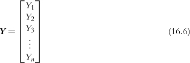
In this case the relationship between the response and the p predictors ( p – 1 predictors and the intercept) is modeled as
where Y is the nx1 response vector
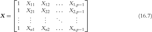
X is the nxp matrix (n rows and p – 1 predictors plus the intercept)
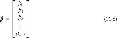
β is the px1 vector of coefficients (one for each predictor and intercept)
and ![]() is the nx1 vector of normally distributed errors
is the nx1 vector of normally distributed errors

with
which seems more complicated than simple regression but the algebra actually gets easier.
The solution for the coefficients is simply written as in Equation 16.11.
To see this in action we use New York City condo evaluations for fiscal year 2011–2012, obtained through NYC Open Data. NYC Open Data is an initiative by New York City to make government more transparent and work better. It provides data on all manner of city services to the public for analysis, scrutiny and app building (through http://nycbigapps.com/). It has been surprisingly popular, spawning hundreds of mobile apps and being copied in other cities such as Chicago and Washington, DC. Its Web site is at https://data.cityofnewyork.us/.
The original data were separated by borough with one file each for Manhattan,2 Brooklyn,3 Queens,4 the Bronx5 and Staten Island,6 and contained extra information we will not be using. So we combined the five files into one, cleaned up the column names and posted it at http://www.jaredlander.com/data/housing.csv. To access the data, either download it from that URL and use read.table on the now local file, or read it directly from the URL.
2. https://data.cityofnewyork.us/Finances/DOF-Condominium-Comparable-Rental-Income-Manhattan/dvzp-h4k9
3. https://data.cityofnewyork.us/Finances/DOF-Condominium-Comparable-Rental-Income-Brooklyn-/bss9-579f
4. https://data.cityofnewyork.us/Finances/DOF-Condominium-Comparable-Rental-Income-Queens-FY/jcih-dj9q
5. https://data.cityofnewyork.us/Property/DOF-Condominium-Comparable-Rental-Income-Bronx-FY-/3qfc-4tta
6. https://data.cityofnewyork.us/Finances/DOF-Condominium-Comparable-Rental-Income-Staten-Is/tkdy-59zg
> housing <- read.table("http://www.jaredlander.com/data/housing.csv",
+ sep = ",", header = TRUE,
+ stringsAsFactors = FALSE)
A few reminders about what that code does: sep specifies that commas were used to separate columns; header means the first row contains the column names; and stringsAsFactors leaves character columns as they are and does not convert them to factors, which speeds up loading time and also makes them easier to work with. Looking at the data, we see that we have a lot of columns and some bad names, so we should rename those.
> names(housing) <- c("Neighborhood", "Class", "Units", "YearBuilt",
+ "SqFt", "Income", "IncomePerSqFt", "Expense",
+ "ExpensePerSqFt", "NetIncome", "Value",
+ "ValuePerSqFt", "Boro")
> head(housing)
Neighborhood Class Units YearBuilt SqFt Income
1 FINANCIAL R9-CONDOMINIUM 42 1920 36500 1332615
2 FINANCIAL R4-CONDOMINIUM 78 1985 126420 6633257
3 FINANCIAL RR-CONDOMINIUM 500 NA 554174 17310000
4 FINANCIAL R4-CONDOMINIUM 282 1930 249076 11776313
5 TRIBECA R4-CONDOMINIUM 239 1985 219495 10004582
6 TRIBECA R4-CONDOMINIUM 133 1986 139719 5127687
IncomePerSqFt Expense ExpensePerSqFt NetIncome Value
1 36.51 342005 9.37 990610 7300000
2 52.47 1762295 13.94 4870962 30690000
3 31.24 3543000 6.39 13767000 90970000
4 47.28 2784670 11.18 8991643 67556006
5 45.58 2783197 12.68 7221385 54320996
6 36.70 1497788 10.72 3629899 26737996
ValuePerSqFt Boro
1 200.00 Manhattan
2 242.76 Manhattan
3 164.15 Manhattan
4 271.23 Manhattan
5 247.48 Manhattan
6 191.37 Manhattan
For this data the response is the value per square foot and the predictors are everything else. However, we ignore the income and expense variables, as they are actually just estimates based on an arcane requirement that condos be compared to rentals for valuation purposes. The first step is to visualize the data in some exploratory data analysis. The natural place to start is with a histogram of ValuePerSqFt, which is shown in Figure 16.3.
> ggplot(housing, aes(x=ValuePerSqFt)) +
+ geom_histogram(binwidth=10) + labs(x="Value per Square Foot")
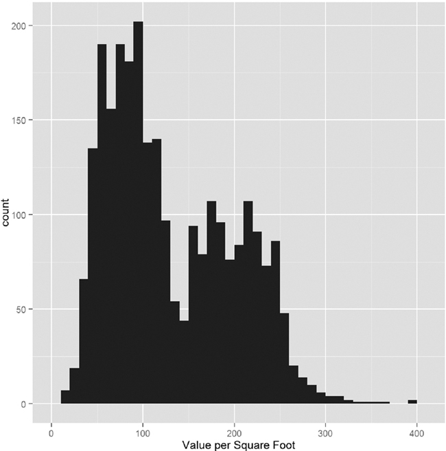
The bimodal nature of the histogram means there is something left to be explored. Mapping color to Boro in Figure 16.4a and faceting on Boro in Figure 16.4b reveal that Brooklyn and Queens make up one mode and Manhattan makes up the other, while there is not much data on the Bronx and Staten Island.
> ggplot(housing, aes(x=ValuePerSqFt, fill=Boro)) +
+ geom_histogram(binwidth=10) + labs(x="Value per Square Foot")
> ggplot(housing, aes(x=ValuePerSqFt, fill=Boro)) +
+ geom_histogram(binwidth=10) + labs(x="Value per Square Foot") +
+ facet_wrap(~Boro)
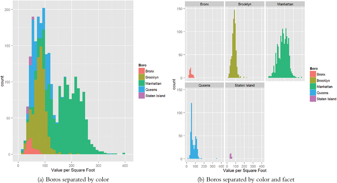
Figure 16.4 Histograms of value per square foot. These illustrate structure in the data revealing that Brooklyn and Queens make up one mode and Manhattan makes up the other, while there is not much data on the Bronx and Staten Island.
Next we should look at histograms for square footage and the number of units.
> ggplot(housing, aes(x=SqFt)) + geom_histogram()
> ggplot(housing, aes(x=Units)) + geom_histogram()
> ggplot(housing[housing$Units < 1000, ],
+ aes(x=SqFt)) + geom_histogram()
> ggplot(housing[housing$Units < 1000, ],
+ aes(x=Units)) + geom_histogram()
Figure 16.5 shows that there are quite a few buildings with an incredible number of units. Plotting scatterplots in Figure 16.6 of the value per square foot versus both number of units and square footage, with and without those outlying buildings, gives us an idea whether we can remove them from the analysis.

Figure 16.5 Histograms for total square feet and number of units. The distributions are highly right skewed in the top two graphs, so they were repeated after removing buildings with more than 1,000 units.
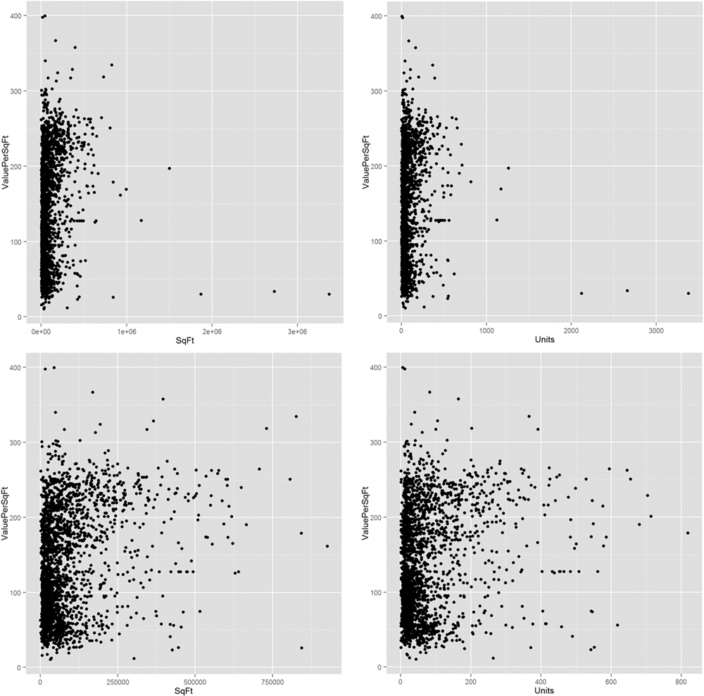
Figure 16.6 Scatterplots of value per square foot versus square footage and value versus number of units, both with and without the buildings that have over 1,000 units.
> ggplot(housing, aes(x = SqFt, y = ValuePerSqFt)) + geom_point()
> ggplot(housing, aes(x = Units, y = ValuePerSqFt)) + geom_point()
> ggplot(housing[housing$Units < 1000, ], aes(x = SqFt,
+ y = ValuePerSqFt)) + geom_point()
> ggplot(housing[housing$Units < 1000, ], aes(x = Units,
+ y = ValuePerSqFt)) + geom_point()
> # how many need to be removed?
> sum(housing$Units >= 1000)
[1] 6
> # remove them
> housing <- housing[housing$Units < 1000, ]
Even after we remove the outliers, it still seems like a log transformation of some data could be helpful. Figures 16.7 and 16.8 show that taking the log of square footage and number of units might prove helpful. It also shows what happens when taking the log of value.
> # plot ValuePerSqFt against SqFt
> ggplot(housing, aes(x=SqFt, y=ValuePerSqFt)) + geom_point()
> ggplot(housing, aes(x=log(SqFt), y=ValuePerSqFt)) + geom_point()
> ggplot(housing, aes(x=SqFt, y=log(ValuePerSqFt))) + geom_point()
> ggplot(housing, aes(x=log(SqFt), y=log(ValuePerSqFt))) +
+ geom_point()
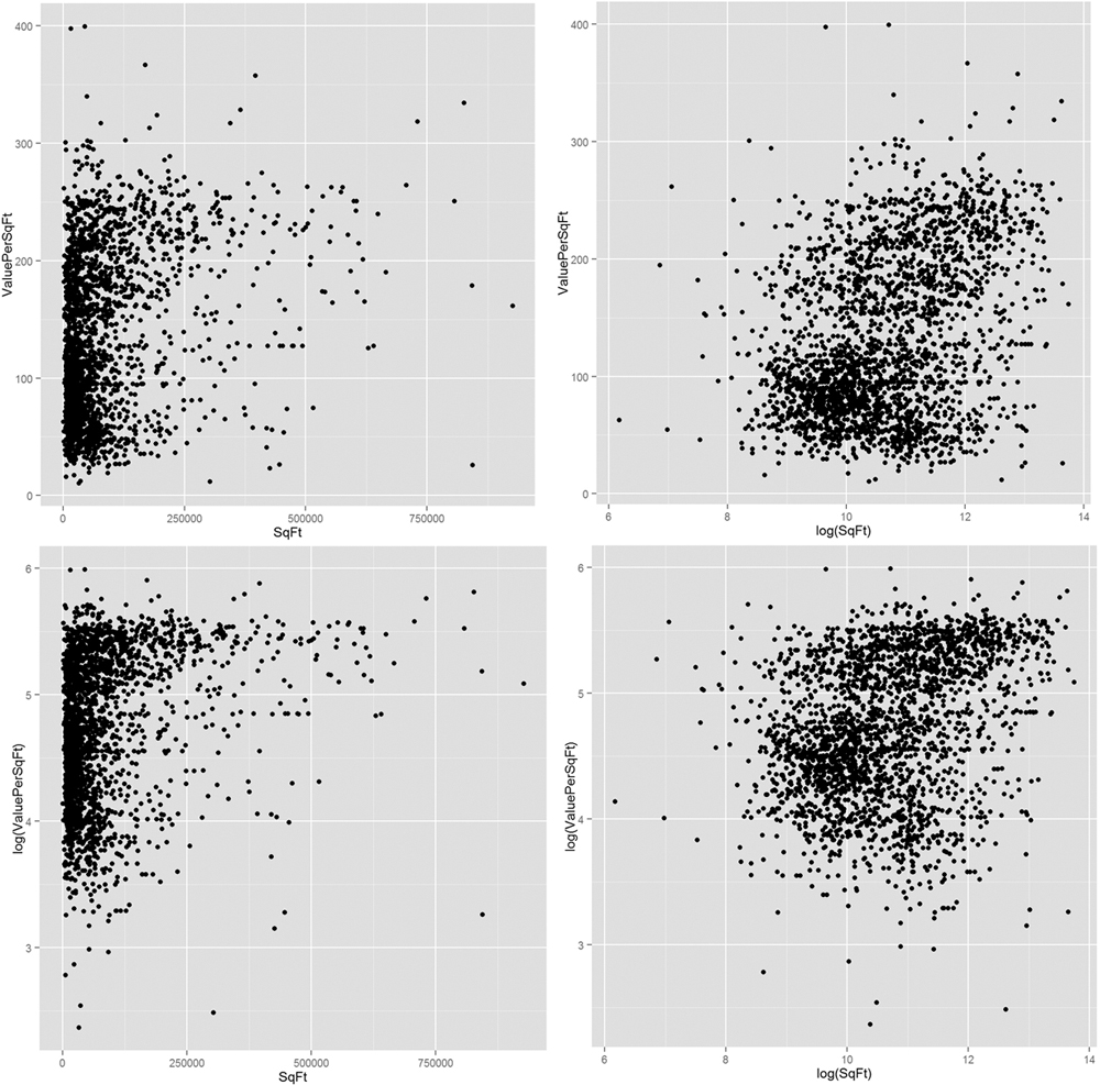
Figure 16.7 Scatterplots of value versus square footage. The plots indicate that taking the log of SqFt might be useful in modeling.
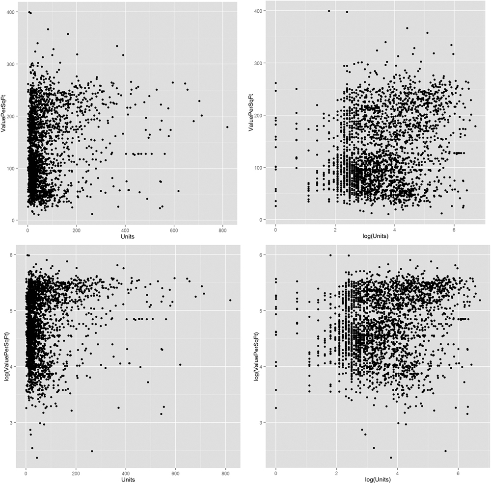
Figure 16.8 Scatterplots of value versus number of units. It is not yet certain whether taking logs will be useful in modeling.
> # plot ValuePerSqFt against Units
> ggplot(housing, aes(x=Units, y=ValuePerSqFt)) + geom_point()
> ggplot(housing, aes(x=log(Units), y=ValuePerSqFt)) + geom_point()
> ggplot(housing, aes(x=Units, y=log(ValuePerSqFt))) + geom_point()
> ggplot(housing, aes(x=log(Units), y=log(ValuePerSqFt))) +
+ geom_point()
Now that we have viewed our data a few different ways, it is time to start modeling. We already saw from Figure 16.4 that accounting for the different boroughs will be important and the various scatterplots indicated that Units and SqFt will be important as well.
Fitting the model uses the formula interface in lm. Now that there are multiple predictors, we separate them on the right side of the formula using plus signs (+).
> house1 <- lm(ValuePerSqFt ~ Units + SqFt + Boro, data = housing)
> summary(house1)
Call:
lm(formula = ValuePerSqFt ~ Units + SqFt + Boro, data = housing)
Residuals:
Min 1Q Median 3Q Max
-168.458 -22.680 1.493 26.290 261.761
Coefficients:
Estimate Std. Error t value Pr(>|t|)
(Intercept) 4.430e+01 5.342e+00 8.293 <2e-16 ***
Units -1.532e-01 2.421e-02 -6.330 2.88e-10 ***
SqFt 2.070e-04 2.129e-05 9.723 < 2e-16 ***
BoroBrooklyn 3.258e+01 5.561e+00 5.858 5.28e-09 ***
BoroManhattan 1.274e+02 5.459e+00 23.343 < 2e-16 ***
BoroQueens 3.011e+01 5.711e+00 5.272 1.46e-07 ***
BoroStaten Island -7.114e+00 1.001e+01 -0.711 0.477
---
Signif. codes: 0 '***' 0.001 '**' 0.01 '*' 0.05 '.' 0.1 ' ' 1
Residual standard error: 43.2 on 2613 degrees of freedom
Multiple R-squared: 0.6034, Adjusted R-squared: 0.6025
F-statistic: 662.6 on 6 and 2613 DF, p-value: < 2.2e-16
The first thing to notice is that in some versions of R there is a message warning us that Boro was converted to a factor. This is because Boro was stored as a character, and for modeling purposes character data must be represented using indicator variables, which is how factors are treated inside modeling functions, as seen on page 60 in Section 5.1.
The summary function prints out information about the model, including how the function was called, quantiles for the residuals, coefficient estimates, standard errors and p-values for each variable, and the degrees of freedom, p-value and F-statistic for the model. There is no coefficient for the Bronx because that is the baseline level of Boro, and all the other Boro coefficients are relative to that baseline.
The coefficients represent the effect of the predictors on the response and the standard errors are the uncertainty in the estimation of the coefficients. The t value (t-statistic) and p-value for the coefficients are numerical measures of statistical significance, though these should be viewed with caution as most modern data scientists do not like to look at the statistical significance of individual coefficients but rather judge the model as a whole as covered in Chapter 18.
The model p-value and F-statistic are measures of its goodness of fit. The degrees of freedom for a regression are calculated as the number of observations minus the number of coefficients. In this example, there are nrow(housing)-length(coef(house1))=2613 degrees of freedom.
A quick way to grab the coefficients from a model is to either use the coef function or get them from the model using the $ operator on the model object.
> house1$coefficients
(Intercept) Units SqFt
4.430325e+01 -1.532405e-01 2.069727e-04
BoroBrooklyn BoroManhattan BoroQueens
3.257554e+01 1.274259e+02 3.011000e+01
BoroStaten Island
-7.113688e+00
> coef(house1)
(Intercept) Units SqFt
4.430325e+01 -1.532405e-01 2.069727e-04
BoroBrooklyn BoroManhattan BoroQueens
3.257554e+01 1.274259e+02 3.011000e+01
BoroStaten Island
-7.113688e+00
> # works the same as coef
> coefficients(house1)
(Intercept) Units SqFt
4.430325e+01 -1.532405e-01 2.069727e-04
BoroBrooklyn BoroManhattan BoroQueens
3.257554e+01 1.274259e+02 3.011000e+01
BoroStaten Island
-7.113688e+00
As a repeated theme, we prefer visualizations over tables of information, and a great way of visualizing regression results is a coefficient plot like the one shown in Figure 16.2. Rather than build it from scratch, we use the convenient coefplot package that we wrote. Figure 16.9 shows the result, where each coefficient is plotted as a point with a thick line representing the one standard error confidence interval and a thin line representing the two standard error confidence interval. There is a vertical line indicating 0. In general, a good rule of thumb is that if the two standard error confidence interval does not contain 0, it is statistically significant.
> require(coefplot)
> coefplot(house1)

Figure 16.9 shows that, as expected, being located in Manhattan has the largest effect on value per square foot. Surprisingly, the number of units or square feet in a building has little effect on value. This is a model with purely additive terms. Interactions between variables can be equally powerful. To enter them in a formula, separate the desired variables with a * instead of +. Doing so results in the individual variables plus the interaction term being included in the model. To include just the interaction term, and not the individual variables, use : instead. The results of interacting Units and SqFt are shown in Figure 16.10.
> house2 <- lm(ValuePerSqFt ~ Units * SqFt + Boro, data = housing)
> house3 <- lm(ValuePerSqFt ~ Units:SqFt + Boro, data = housing)
> house2$coefficients
(Intercept) Units SqFt
4.093685e+01 -1.024579e-01 2.362293e-04
BoroBrooklyn BoroManhattan BoroQueens
3.394544e+01 1.272102e+02 3.040115e+01
BoroStaten Island Units:SqFt
-8.419682e+00 -1.809587e-07
> house3$coefficients
(Intercept) BoroBrooklyn BoroManhattan
4.804972e+01 3.141208e+01 1.302084e+02
BoroQueens BoroStaten Island Units:SqFt
2.841669e+01 -7.199902e+00 1.088059e-07
> coefplot(house2)
> coefplot(house3)

Figure 16.10 Coefficient plots for models with interaction terms. (a) includes individual variables and the interaction term, while (b) only includes the interaction term.
If three variables all interact together, the resulting coefficients will be the three individual terms, three two-way interactions and one three-way interaction.
> house4 <- lm(ValuePerSqFt ~ SqFt * Units * Income, housing)
> house4$coefficients
(Intercept) SqFt Units
1.116433e+02 -1.694688e-03 7.142611e-03
Income SqFt:Units SqFt:Income
7.250830e-05 3.158094e-06 -5.129522e-11
Units:Income SqFt:Units:Income
-1.279236e-07 9.107312e-14
Interacting (from now on, unless otherwise specified, interacting will refer to the * operator) a continuous variable like SqFt with a factor like Boro results in individual terms for the continuous variable and each non-baseline level of the factor plus an interaction term between the continuous variable and each non-baseline level of the factor. Interacting two (or more) factors yields terms for all the individual non-baseline levels in both factors and an interaction term for every combination of non-baseline levels of the factors.
> house5 <- lm(ValuePerSqFt ~ Class * Boro, housing)
> house5$coefficients
(Intercept)
47.041481
ClassR4-CONDOMINIUM
4.023852
ClassR9-CONDOMINIUM
-2.838624
ClassRR-CONDOMINIUM
3.688519
BoroBrooklyn
27.627141
BoroManhattan
89.598397
BoroQueens
19.144780
BoroStaten Island
-9.203410
ClassR4-CONDOMINIUM:BoroBrooklyn
4.117977
ClassR9-CONDOMINIUM:BoroBrooklyn
2.660419
ClassRR-CONDOMINIUM:BoroBrooklyn
-25.607141
ClassR4-CONDOMINIUM:BoroManhattan
47.198900
ClassR9-CONDOMINIUM:BoroManhattan
33.479718
ClassRR-CONDOMINIUM:BoroManhattan
10.619231
ClassR4-CONDOMINIUM:BoroQueens
13.588293
ClassR9-CONDOMINIUM:BoroQueens
-9.830637
ClassRR-CONDOMINIUM:BoroQueens
34.675220
ClassR4-CONDOMINIUM:BoroStaten Island
NA
ClassR9-CONDOMINIUM:BoroStaten Island
NA
ClassRR-CONDOMINIUM:BoroStaten Island
NA
Because neither SqFt nor Units appears to be significant in any model, it would be good to test their ratio. To simply divide one variable by another in a formula, the division must be wrapped in the I function.
> house6 <- lm(ValuePerSqFt ~ I(SqFt/Units) + Boro, housing)
> house6$coefficients
(Intercept) I(SqFt/Units) BoroBrooklyn
43.754838763 0.004017039 30.774343209
BoroManhattan BoroQueens BoroStaten Island
130.769502685 29.767922792 -6.134446417
The I function is used to preserve a mathematical relationship in a formula and prevent it from being interpreted according to formula rules. For instance, using (Units + SqFt)^2 in a formula is the same as using Units * SqFt, whereas I(Units + SqFt)^2 will include the square of the sum of the two variables as a term in the formula.
> house7 <- lm(ValuePerSqFt ~ (Units + SqFt)^2, housing)
> house7$coefficients
(Intercept) Units SqFt Units:SqFt
1.070301e+02 -1.125194e-01 4.964623e-04 -5.159669e-07
> house8 <- lm(ValuePerSqFt ~ Units * SqFt, housing)
> identical(house7$coefficients, house8$coefficients)
[1] TRUE
> house9 <- lm(ValuePerSqFt ~ I(Units + SqFt)^2, housing)
> house9$coefficients
(Intercept) I(Units + SqFt)
1.147034e+02 2.107231e-04
We have fit numerous models from which we need to pick the “best” one. Model selection is discussed in Section 18.2. In the meantime, visualizing the coefficients from multiple models is a handy tool. Figure 16.11 shows a coefficient plot for models house1, house2 and house3.
> # also from the coefplot package
> multiplot(house1, house2, house3)

Figure 16.11 Coefficient plot for multiple condo models. The coefficients are plotted in the same spot on the y-axis for each model. If a model does not contain a particular coefficient, it is simply not plotted.
Regression is often used for prediction, which in R is enabled by the predict function. For this example, new data are available at http://www.jaredlander.com/data/housingNew.csv.
> housingNew <- read.table("http://www.jaredlander.com/data/
+ housingNew.csv", sep = ",", header = TRUE, stringsAsFactors = FALSE)
Making the prediction can be as simple as calling predict, although caution must be used when dealing with factor predictors to ensure that they have the same levels as those used in building the model.
> # make prediction with new data and 95% confidence bounds
> housePredict <- predict(house1, newdata = housingNew, se.fit = TRUE,
+ interval = "prediction", level = .95)
> # view predictions with upper and lower bounds based on
> # standard errors
> head(housePredict$fit)
fit lwr upr
1 74.00645 -10.813887 158.8268
2 82.04988 -2.728506 166.8283
3 166.65975 81.808078 251.5114
4 169.00970 84.222648 253.7968
5 80.00129 -4.777303 164.7799
6 47.87795 -37.480170 133.2361
> # view the standard errors for the prediction
> head(housePredict$se.fit)
1 2 3 4 5 6
2.118509 1.624063 2.423006 1.737799 1.626923 5.318813
16.3. Conclusion
Perhaps one of the most versatile tools in statistical analysis, regression is well handled using R’s lm function. It takes the formula interface, where a response is modeled on a set of predictors. Other useful arguments to the function are weights, which specifies the weights attributed to observations (both probability and count weights), and subset, which will fit the model only on a subset of the data.