
Chapter 17. Generalized Linear Models
Not all data can be appropriately modeled with linear regression, because they are binomial (TRUE/FALSE) data, count data or some other form. To model these types of data, generalized linear models were developed. They are still modeled using a linear predictor, Xβ, but they are transformed using some link function. To the R user, fitting a generalized linear model requires barely any more effort than running a linear regression.
17.1. Logistic Regression
A very powerful and common model—especially in fields such as marketing and medicine—is logistic regression. The examples in this section will use a subset of data from the 2010 American Community Survey (ACS) for New York State.1 ACS data contain a lot of information, so we have made a subset of it with 22,745 rows and 18 columns available at http://jaredlander.com/data/acs_ny.csv.
1. The ACS is a large-scale survey very similar to the decennial census, except that is conducted on a more frequent basis.
> acs <- read.table("http://jaredlander.com/data/acs_ny.csv", sep = ",",
+ header = TRUE, stringsAsFactors = FALSE)
Logistic regression models are formulated as
where yi is the ith response and Xiβ is the linear predictor. The inverse logit function
transforms the continuous output from the linear predictor to fall between 0 and 1. This is the inverse of the link function.
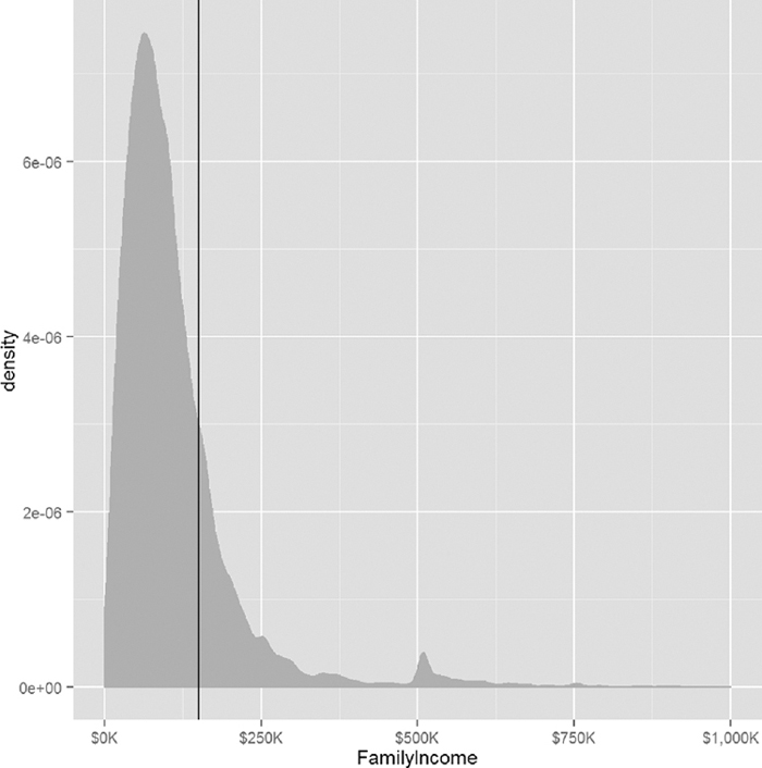
We now formulate a question that asks whether a household has an income greater than $150,000 (See Figure 17.1). To do this we need to create a new binary variable with TRUE for income above that mark and FALSE for income below.
> acs$Income <- with(acs, FamilyIncome >= 150000)
> require(ggplot2)
> require(useful)
> ggplot(acs, aes(x=FamilyIncome)) +
+ geom_density(fill="grey", color="grey") +
+ geom_vline(xintercept=150000) +
+ scale_x_continuous(label=multiple.dollar, limits=c(0, 1000000))
> head(acs)
Acres FamilyIncome FamilyType NumBedrooms NumChildren NumPeople
1 1-10 150 Married 4 1 3
2 1-10 180 Female Head 3 2 4
3 1-10 280 Female Head 4 0 2
4 1-10 330 Female Head 2 1 2
5 1-10 330 Male Head 3 1 2
6 1-10 480 Male Head 0 3 4
NumRooms NumUnits NumVehicles NumWorkers OwnRent
1 9 Single detached 1 0 Mortgage
2 6 Single detached 2 0 Rented
3 8 Single detached 3 1 Mortgage
4 4 Single detached 1 0 Rented
5 5 Single attached 1 0 Mortgage
6 1 Single detached 0 0 Rented
YearBuilt HouseCosts ElectricBill FoodStamp HeatingFuel Insurance
1 1950-1959 1800 90 No Gas 2500
2 Before 1939 850 90 No Oil 0
3 2000-2004 2600 260 No Oil 6600
4 1950-1959 1800 140 No Oil 0
5 Before 1939 860 150 No Gas 660
6 Before 1939 700 140 No Gas 0
Language Income
1 English FALSE
2 English FALSE
3 Other European FALSE
4 English FALSE
5 Spanish FALSE
6 English FALSE
Running a logistic regression is done very similarly to running a linear regression. It still uses the formula interface but the function is glm rather than lm (glm can actually fit linear regressions as well), and a few more options need to be set.
> income1 <- glm(Income ~ HouseCosts + NumWorkers + OwnRent +
+ NumBedrooms + FamilyType,
+ data=acs, family=binomial(link="logit"))
> summary(income1)
Call:
glm(formula = Income ~ HouseCosts + NumWorkers + OwnRent + NumBedrooms +
FamilyType, family = binomial(link = "logit"), data = acs)
Deviance Residuals:
Min 1Q Median 3Q Max
-2.8452 -0.6246 -0.4231 -0.1743 2.9503
Coefficients:
Estimate Std. Error z value Pr(>|z|)
(Intercept) -5.738e+00 1.185e-01 -48.421 <2e-16 ***
HouseCosts 7.398e-04 1.724e-05 42.908 <2e-16 ***
NumWorkers 5.611e-01 2.588e-02 21.684 <2e-16 ***
OwnRentOutright 1.772e+00 2.075e-01 8.541 <2e-16 ***
OwnRentRented -8.886e-01 1.002e-01 -8.872 <2e-16 ***
NumBedrooms 2.339e-01 1.683e-02 13.895 <2e-16 ***
FamilyTypeMale Head 3.336e-01 1.472e-01 2.266 0.0235 *
FamilyTypeMarried 1.405e+00 8.704e-02 16.143 <2e-16 ***
---
Signif. codes: 0 '***' 0.001 '**' 0.01 '*' 0.05 '.' 0.1 ' ' 1
(Dispersion parameter for binomial family taken to be 1)
Null deviance: 22808 on 22744 degrees of freedom
Residual deviance: 18073 on 22737 degrees of freedom
AIC: 18089
Number of Fisher Scoring iterations: 6
> require(coefplot)
> coefplot(income1)

Figure 17.2 Coefficient plot for logistic regression on family income greater than $150,000, based on the American Community Survey.
The output from summary and coefplot for glm is similar to that of lm. There are coefficient estimates, standard errors, p-values—both overall and for the coefficients—and a measure of correctness, which in this case is the deviance and AIC. A general rule of thumb is that adding a variable (or a level of a factor) to a model should result in a drop in deviance of two; otherwise, the variable is not useful in the model. Interactions and all the other formula concepts work the same.
Interpreting the coefficients from a logistic regression necessitates taking the inverse logit.
> invlogit <- function(x)
+ {
+ 1/(1 + exp(-x))
+ }
> invlogit(income1$coefficients)
(Intercept) HouseCosts NumWorkers
0.003211572 0.500184950 0.636702036
OwnRentOutright OwnRentRented NumBedrooms
0.854753527 0.291408659 0.558200010
FamilyTypeMale Head FamilyTypeMarried
0.582624773 0.802983719
17.2. Poisson Regression
Another popular member of the generalized linear models is Poisson regression, which, much like the Poisson distribution, is used for count data. It, like all other generalized linear models, is called using glm. To illustrate we continue using the ACS data with the number of children (NumChildren) as the response.
The formulation for Poisson regression is
where yi is the ith response and
is the mean of the distribution for the ith observation.
Before fitting a model, we look at the histogram of the number of children in each household.
> ggplot(acs, aes(x = NumChildren)) + geom_histogram(binwidth = 1)
While Figure 17.3 does not show data that have a perfect Poisson distribution it is close enough to fit a good model. The coefficient plot is shown in Figure 17.4.
> children1 <- glm(NumChildren ~ FamilyIncome + FamilyType + OwnRent,
+ data=acs, family=poisson(link="log"))
> summary(children1)
Call:
glm(formula = NumChildren ~ FamilyIncome + FamilyType + OwnRent,
family = poisson(link = "log"), data = acs)
Deviance Residuals:
Min 1Q Median 3Q Max
-1.9950 -1.3235 -1.2045 0.9464 6.3781
Coefficients:
Estimate Std. Error z value Pr(>|z|)
(Intercept) -3.257e-01 2.103e-02 -15.491 < 2e-16 ***
FamilyIncome 5.420e-07 6.572e-08 8.247 < 2e-16 ***
FamilyTypeMale Head -6.298e-02 3.847e-02 -1.637 0.102
FamilyTypeMarried 1.440e-01 2.147e-02 6.707 1.98e-11 ***
OwnRentOutright -1.974e+00 2.292e-01 -8.611 < 2e-16 ***
OwnRentRented 4.086e-01 2.067e-02 19.773 < 2e-16 ***
---
Signif. codes: 0 '***' 0.001 '**' 0.01 '*' 0.05 '.' 0.1 ' ' 1
(Dispersion parameter for poisson family taken to be 1)
Null deviance: 35240 on 22744 degrees of freedom
Residual deviance: 34643 on 22739 degrees of freedom
AIC: 61370
Number of Fisher Scoring iterations: 5
> coefplot(children1)

Figure 17.3 Histogram of the number of children per household from the American Community Survey. The distribution is not perfectly Poisson but it is sufficiently so for modeling with Poisson regression.

The output here is similar to that for logistic regression, and the same rule of thumb for deviance applies.
A particular concern with Poisson regression is overdispersion, which means that the variability seen in the data is greater than is theorized by the Poisson distribution where the mean and variance are the same.
Overdispersion is defined as


are the studentized residuals.
Calculating overdispersion in R is as follows.
> # the standardized residuals
> z <- (acs$NumChildren - children1$fitted.values) /
+ sqrt(children1$fitted.values)
> # Overdispersion Factor
> sum(z^2) / children1$df.residual
[1] 1.469747
> # Overdispersion p-value
> pchisq(sum(z^2), children1$df.residual)
[1] 1
Generally an overdispersion ratio of 2 or greater indicates overdispersion. While this overdispersion ratio is less than 2, the p-value is 1, meaning that there is a statistically significant overdispersion. So we refit the model to account for the overdispersion using the quasipoisson family, which actually uses the negative binomial distribution.
> children2 <- glm(NumChildren ~ FamilyIncome + FamilyType + OwnRent,
+ data=acs, family=quasipoisson(link="log"))
> multiplot(children1, children2)
Figure 17.5 shows a coefficient plot for a model that accounts for overdispersion and one that does not. Since the overdispersion was not very large, the second model adds just a little uncertainty to the coefficient estimates.

Figure 17.5 Coefficient plot for Poisson models. The first model, children1, does not account for overdispersion, while children2 does. Because the overdispersion was not too big, the coefficient estimates in the second model have just a bit more uncertainty.
17.3. Other Generalized Linear Models
Other common generalized linear models supported by the glm function are gamma, inverse gaussian and quasibinomial. Different link functions can be supplied, such as the following: logit, probit, cauchit, log and cloglog for binomial; inverse, identity and log for gamma; log, identity and sqrt for Poisson; and 1/mu^2, inverse, identity and log for inverse gaussian.
Multinomial regression, for classifying multiple categories, requires either running multiple logistic regressions (a tactic well supported in statistical literature) or using the polr function or the multinom function from the nnet package.
17.4. Survival Analysis
While not technically part of the family of generalized linear models, survival analysis is another important extension to regression. It has many applications, such as clinical medical trials, server failure times, number of accidents and time to death after a treatment or disease.
Data used for survival analysis are different from most other data in that they are censored, meaning there is unknown information, typically about what happens to a subject after a given amount of time. For an example, we look at the bladder data from the survival package.
> require(survival)
> head(bladder)
id rx number size stop event enum
1 1 1 1 3 1 0 1
2 1 1 1 3 1 0 2
3 1 1 1 3 1 0 3
4 1 1 1 3 1 0 4
5 2 1 2 1 4 0 1
6 2 1 2 1 4 0 2
The columns of note are stop (when an event occurs or the patient leaves the study) and event (whether an event occurred at the time). Even if event is 0, we do not know if an event could have occurred later; this is why it is called censored. Making use of that structure requires the Surv function.
> # first look at a piece of the data
> bladder[100:105, ]
id rx number size stop event enum
100 25 1 2 1 12 1 4
101 26 1 1 3 12 1 1
102 26 1 1 3 15 1 2
103 26 1 1 3 24 1 3
104 26 1 1 3 31 0 4
105 27 1 1 2 32 0 1
> # now look at the response variable built by build.y
> survObject <- with(bladder[100:105, ], Surv(stop, event))
> # nicely printed form
> survObject
[1] 12 12 15 24 31+ 32+
> # see its matrix form
> survObject[, 1:2]
time status
[1,] 12 1
[2,] 12 1
[3,] 15 1
[4,] 24 1
[5,] 31 0
[6,] 32 0
This shows that for the first three rows where an event occurred, the time is known to be 12, whereas the bottom two rows had no event, so the time is censored because an event could have occurred afterward.
Perhaps the most common modeling technique in survival analysis is using a Cox proportional hazards model, which in R is done with coxph. The model is fitted using the familiar formula interface supplied to coxph. The survfit function builds the survival curve that can then be plotted as shown in Figure 17.6. The survival curve shows the percentage of participants surviving at a given time. The summary is similar to other summaries but tailored to survival analysis.
> cox1 <- coxph(Surv(stop, event) ~ rx + number + size + enum,
+ data=bladder)
> summary(cox1)
Call:
coxph(formula = Surv(stop, event) ~ rx + number + size + enum,
data = bladder)
n= 340, number of events= 112
coef exp(coef) se(coef) z Pr(>|z|)
rx -0.59739 0.55024 0.20088 -2.974 0.00294 **
number 0.21754 1.24301 0.04653 4.675 2.93e-06 ***
size -0.05677 0.94481 0.07091 -0.801 0.42333
enum -0.60385 0.54670 0.09401 -6.423 1.34e-10 ***
---
Signif. codes: 0 '***' 0.001 '**' 0.01 '*' 0.05 '.' 0.1 ' ' 1
exp(coef) exp(-coef) lower .95 upper .95
rx 0.5502 1.8174 0.3712 0.8157
number 1.2430 0.8045 1.1347 1.3617
size 0.9448 1.0584 0.8222 1.0857
enum 0.5467 1.8291 0.4547 0.6573
Concordance= 0.753 (se = 0.029 )
Rsquare= 0.179 (max possible= 0.971 )
Likelihood ratio test= 67.21 on 4 df, p=8.804e-14
Wald test = 64.73 on 4 df, p=2.932e-13
Score (logrank) test = 69.42 on 4 df, p=2.998e-14
> plot(survfit(cox1), xlab="Days", ylab="Survival Rate",
+ conf.int=TRUE)

In this data, the rx variable indicates placebo versus treatment, which is a natural stratification of the patients. Passing rx to strata in the formula splits the data into two for analysis and will result in two survival curves like those in Figure 17.7.
> cox2 <- coxph(Surv(stop, event) ~ strata(rx) + number + size + enum,
+ data=bladder)
> summary(cox2)
Call:
coxph(formula = Surv(stop, event) ~ strata(rx) + number + size +
enum, data = bladder)
n= 340, number of events= 112
coef exp(coef) se(coef) z Pr(>|z|)
number 0.21371 1.23826 0.04648 4.598 4.27e-06 ***
size -0.05485 0.94662 0.07097 -0.773 0.44
enum -0.60695 0.54501 0.09408 -6.451 1.11e-10 ***
---
Signif. codes: 0 '***' 0.001 '**' 0.01 '*' 0.05 '.' 0.1 ' ' 1
exp(coef) exp(-coef) lower .95 upper .95
number 1.2383 0.8076 1.1304 1.3564
size 0.9466 1.0564 0.8237 1.0879
enum 0.5450 1.8348 0.4532 0.6554
Concordance= 0.74 (se = 0.04 )
Rsquare= 0.166 (max possible= 0.954 )
Likelihood ratio test= 61.84 on 3 df, p=2.379e-13
Wald test = 60.04 on 3 df, p=5.751e-13
Score (logrank) test = 65.05 on 3 df, p=4.896e-14
> plot(survfit(cox2), xlab="Days", ylab="Survival Rate",
+ conf.int=TRUE, col=1:2)
> legend("bottomleft", legend=c(1, 2), lty=1, col=1:2,
+ text.col=1:2, title="rx")

Figure 17.7 Survival curve for Cox proportional hazards model fitted on bladder data stratified on rx.
As an aside, this was a relatively simple legend to produce but it took a lot more effort than it would with ggplot2.
Testing the assumption of proportional hazards is done with cox.zph.
> cox.zph(cox1)
rho chisq p
rx 0.0299 0.0957 7.57e-01
number 0.0900 0.6945 4.05e-01
size -0.1383 2.3825 1.23e-01
enum 0.4934 27.2087 1.83e-07
GLOBAL NA 32.2101 1.73e-06
> cox.zph(cox2)
rho chisq p
number 0.0966 0.785 3.76e-01
size -0.1331 2.197 1.38e-01
enum 0.4972 27.237 1.80e-07
GLOBAL NA 32.101 4.98e-07
An Andersen-Gill analysis is similar to survival analysis, except it takes intervalized data and can handle multiple events such as counting the number of emergency room visits as opposed to whether or not there is an emergency room visit. It is also performed using coxph, except an additional variable is passed to Surv, and the data must be clustered on an identification column (id) to keep track of multiple events. The corresponding survival curves are seen in Figure 17.8.
> head(bladder2)
id rx number size start stop event enum
1 1 1 1 3 0 1 0 1
2 2 1 2 1 0 4 0 1
3 3 1 1 1 0 7 0 1
4 4 1 5 1 0 10 0 1
5 5 1 4 1 0 6 1 1
6 5 1 4 1 6 10 0 2
> ag1 <- coxph(Surv(start, stop, event) ~ rx + number + size + enum +
+ cluster(id), data=bladder2)
> ag2 <- coxph(Surv(start, stop, event) ~ strata(rx) + number + size +
+ enum + cluster(id), data=bladder2)
> plot(survfit(ag1), conf.int=TRUE)
> plot(survfit(ag2), conf.int=TRUE, col=1:2)
> legend("topright", legend=c(1, 2), lty=1, col=1:2,
+ text.col=1:2, title="rx")

17.5. Conclusion
Generalized linear models extend regression beyond linear relationships between the predictors and response. The most prominent types are logistic for binary data, Poisson for count data and survival analysis. Their uses go far beyond that, but those are by far the most common.