
Chapter 18. Model Diagnostics
Building a model can be a never-ending process in which we constantly improve the model by adding interactions, taking away variables, doing transformations and so on. However, at some point we need to confirm that we have the best model at the time, or even a good model. That leads to the question: How do we judge the quality of a model? In almost all cases the answer has to be: in relation to other models. This could be an analysis of residuals, the results of an ANOVA test or a Wald test, drop-in deviance, the AIC or BIC score, cross-validation error or bootstrapping.
18.1. Residuals
One of the first-taught ways of assessing model quality is an analysis of the residuals, which is the difference between the actual response and the fitted values, values predicted by the model. This is a direct result of the formulation in Equation 16.1 where the errors, akin to residuals, are normally distributed. The basic idea is that if the model is appropriately fitted to the data, the residuals should be normally distributed as well. To see this, we start with the housing data to which we fit a regression and visualize with a coefficient plot, as shown in Figure 18.1.
> # read in the data
> housing <- read.table("data/housing.csv", sep=",", header=TRUE,
+ stringsAsFactors=FALSE)
> # give the data good names
> names(housing) <- c("Neighborhood", "Class", "Units", "YearBuilt",
+ "SqFt", "Income", "IncomePerSqFt", "Expense",
+ "ExpensePerSqFt", "NetIncome", "Value",
+ "ValuePerSqFt", "Boro")
> # eliminate some outliers
> housing <- housing[housing$Units < 1000, ]
> head(housing)
Neighborhood Class Units YearBuilt SqFt Income
1 FINANCIAL R9-CONDOMINIUM 42 1920 36500 1332615
2 FINANCIAL R4-CONDOMINIUM 78 1985 126420 6633257
3 FINANCIAL RR-CONDOMINIUM 500 NA 554174 17310000
4 FINANCIAL R4-CONDOMINIUM 282 1930 249076 11776313
5 TRIBECA R4-CONDOMINIUM 239 1985 219495 10004582
6 TRIBECA R4-CONDOMINIUM 133 1986 139719 5127687
IncomePerSqFt Expense ExpensePerSqFt NetIncome Value
1 36.51 342005 9.37 990610 7300000
2 52.47 1762295 13.94 4870962 30690000
3 31.24 3543000 6.39 13767000 90970000
4 47.28 2784670 11.18 8991643 67556006
5 45.58 2783197 12.68 7221385 54320996
6 36.70 1497788 10.72 3629899 26737996
ValuePerSqFt Boro
1 200.00 Manhattan
2 242.76 Manhattan
3 164.15 Manhattan
4 271.23 Manhattan
5 247.48 Manhattan
6 191.37 Manhattan
>
> # fit a model
> house1 <- lm(ValuePerSqFt ~ Units + SqFt + Boro, data=housing)
> summary(house1)
Call:
lm(formula = ValuePerSqFt ~ Units + SqFt + Boro, data = housing)
Residuals:
Min 1Q Median 3Q Max
-168.458 -22.680 1.493 26.290 261.761
Coefficients:
Estimate Std. Error t value Pr(>|t|)
(Intercept) 4.430e+01 5.342e+00 8.293 < 2e-16 ***
Units -1.532e-01 2.421e-02 -6.330 2.88e-10 ***
SqFt 2.070e-04 2.129e-05 9.723 < 2e-16 ***
BoroBrooklyn 3.258e+01 5.561e+00 5.858 5.28e-09 ***
BoroManhattan 1.274e+02 5.459e+00 23.343 < 2e-16 ***
BoroQueens 3.011e+01 5.711e+00 5.272 1.46e-07 ***
BoroStaten Island -7.114e+00 1.001e+01 -0.711 0.477
---
Signif. codes: 0 '***' 0.001 '**' 0.01 '*' 0.05 '.' 0.1 ' ' 1
Residual standard error: 43.2 on 2613 degrees of freedom
Multiple R-squared: 0.6034, Adjusted R-squared: 0.6025
F-statistic: 662.6 on 6 and 2613 DF, p-value: <2.2e-16
>
> # visualize the model
> require(coefplot)
> coefplot(house1)

For linear regression, three important residual plots are fitted values against residuals, Q-Q plots and the histogram of the residuals. The first is easy enough with ggplot2. Fortunately, ggplot2 has a handy trick for dealing with lm models. We can use the model as the data source and ggplot2 “fortifies” it, creating new columns, for easy plotting.
> require(ggplot2)
> # see what a fortified lm model looks like
> head(fortify(house1))
ValuePerSqFt Units SqFt Boro .hat .sigma
1 200.00 42 36500 Manhattan 0.0009594821 43.20952
2 242.76 78 126420 Manhattan 0.0009232393 43.19848
3 164.15 500 554174 Manhattan 0.0089836758 43.20347
4 271.23 282 249076 Manhattan 0.0035168641 43.17583
5 247.48 239 219495 Manhattan 0.0023865978 43.19289
6 191.37 133 139719 Manhattan 0.0008934957 43.21225
.cooksd .fitted .resid .stdresid
1 5.424169e-05 172.8475 27.15248 0.6287655
2 2.285253e-04 185.9418 56.81815 1.3157048
3 1.459368e-03 209.8077 -45.65775 -1.0615607
4 2.252653e-03 180.0672 91.16278 2.1137487
5 8.225193e-04 180.5341 66.94589 1.5513636
6 8.446170e-06 180.2661 11.10385 0.2571216
> # save a plot to an object
> # notice we are using the created columns for the x- and y-axes
> # they are .fitted and .resid
> h1 <- ggplot(aes(x=.fitted, y=.resid), data = house1) +
+ geom_point() +
+ geom_hline(yintercept = 0) +
+ geom_smooth(se = FALSE) +
+ labs(x="Fitted Values", y="Residuals")
>
> # print the plot
> h1
The plot of residuals versus fitted values shown in Figure 18.2 is at first glance disconcerting, because the pattern in the residuals shows that they are not as randomly dispersed as desired. However, further investigation reveals that this is due to the structure that Boro gives the data, as seen in Figure 18.3.
> h1 + geom_point(aes(color = Boro))

Figure 18.2 Plot of residuals versus fitted values for house1. This clearly shows a pattern in the data that does not appear to be random.
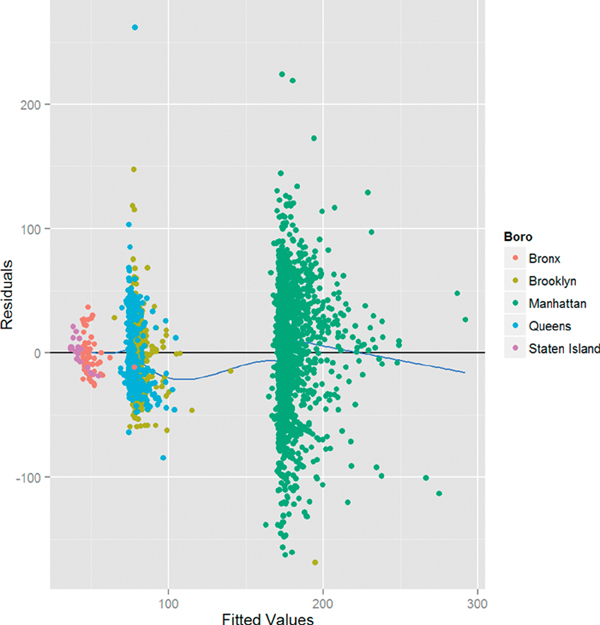
Figure 18.3 Plot of residuals versus fitted values for house1 colored by Boro. The pattern in the residuals is revealed to be the result of the effect of Boro on the model. Notice that the points sit above the x-axis and the smoothing curve because geom point was added after the other geoms, meaning it gets layered on top.
This plot could have been easily, although less attractively, plotted using the built-in plotting function, as shown in Figure 18.4.
> # basic plot
> plot(house1, which=1)
> # same plot but colored by Boro
> plot(house1, which=1, col=as.numeric(factor(house1$model$Boro)))
> # corresponding legend
> legend("topright", legend=levels(factor(house1$model$Boro)), pch=1,
+ col=as.numeric(factor(levels(factor(house1$model$Boro)))),
+ text.col=as.numeric(factor(levels(factor(house1$model$Boro)))),
+ title="Boro")

Next up is the Q-Q plot. If the model is a good fit, the standardized residuals should all fall along a straight line when plotted against the theoretical quantiles of the normal distribution. Both the base graphics and ggplot2 versions are shown in Figure 18.5.
> plot(house1, which = 2)
> ggplot(house1, aes(sample = .stdresid)) + stat_qq() + geom_abline()
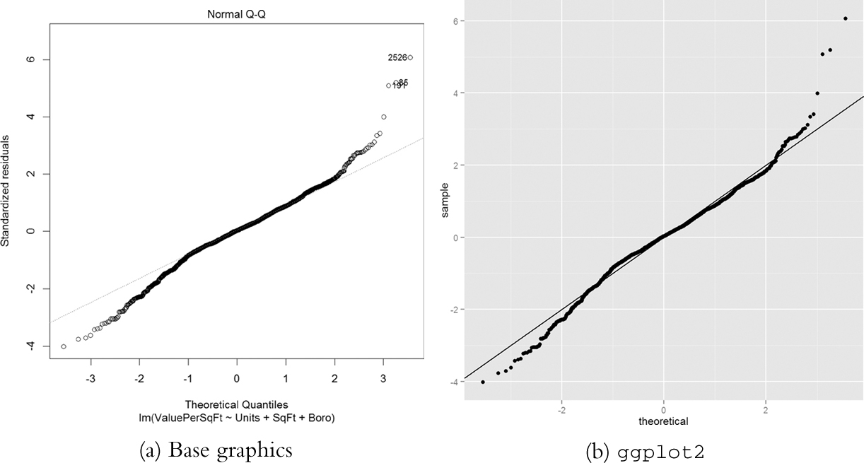
Figure 18.5 Q-Q plot for house1. The tails drift away from the ideal theoretical line, indicating that we do not have the best fit.
Another diagnostic is a histogram of the residuals. This time we will not be showing the base graphics alternative because a histogram is a standard plot that we have shown repeatedly. The histogram in Figure 18.6 is not normally distributed, meaning that our model is not an entirely correct specification.
> ggplot(house1, aes(x = .resid)) + geom_histogram()

Figure 18.6 Histogram of residuals from house1. This does not look normally distributed, meaning our model is incomplete.
18.2. Comparing Models
All of this measuring of model fit only really makes sense when comparing multiple models, because all of these measures are relative. So we will fit a number of models in order to compare them to each other.
> house2 <- lm(ValuePerSqFt ~ Units * SqFt + Boro, data=housing)
> house3 <- lm(ValuePerSqFt ~ Units + SqFt * Boro + Class,
+ data=housing)
> house4 <- lm(ValuePerSqFt ~ Units + SqFt * Boro + SqFt*Class,
+ data=housing)
> house5 <- lm(ValuePerSqFt ~ Boro + Class, data=housing)
As usual, our first step is to visualize the models together using multiplot from the coefplot package. The result is in Figure 18.7 and shows that Boro is the only variable with a significant effect on ValuePerSqFt as do certain condominium types.
> multiplot(house1, house2, house3, house4, house5, pointSize = 2)
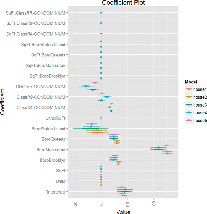
Figure 18.7 Coefficient plot of various models based on housing data. This shows that only Boro and some condominium types matter.
While we do not promote using ANOVA for a multisample test, we do believe it serves a useful purpose in testing the relative merits of different models. Simply passing multiple model objects to anova will return a table of results including the residual sum of squares (RSS), which is a measure of error, the lower the better.
> anova(house1, house2, house3, house4, house5)
Analysis of Variance Table
Model 1: ValuePerSqFt ~ Units + SqFt + Boro
Model 2: ValuePerSqFt ~ Units * SqFt + Boro
Model 3: ValuePerSqFt ~ Units + SqFt * Boro + Class
Model 4: ValuePerSqFt ~ Units + SqFt * Boro + SqFt * Class
Model 5: ValuePerSqFt ~ Boro + Class
Res.Df RSS Df Sum of Sq F Pr(>F)
1 2613 4877506
2 2612 4847886 1 29620 17.0360 3.783e-05 ***
3 2606 4576769 6 271117 25.9888 < 2.2e-16 ***
4 2603 4525783 3 50986 9.7749 2.066e-06 ***
5 2612 4895630 -9 -369847 23.6353 < 2.2e-16 ***
---
Signif. codes: 0 '***' 0.001 '**' 0.01 '*' 0.05 '.' 0.1 ' ' 1
This shows that the fourth model, house4, has the lowest RSS, meaning it is the best model of the bunch. The problem with RSS is that it always improves when an additional variable is added to the model. This can lead to excessive model complexity and overfitting. Another metric, which penalizes model complexity, is the Akaike Information Criterion (AIC). As with RSS, the model with the lowest AIC—even negative values—is considered optimal. The BIC (Bayesian Information Criterion) is a similar measure where, once again, lower is better.
The formula for AIC is
where ln (![]() ) is the maximized log-likelihood and p is the number of coefficients in the model. As the model improves the log-likelihood gets bigger, and because that term is negated the AIC gets lower. However, adding coefficients increases the AIC; this penalizes model complexity. The formula for BIC is similar except that instead of multiplying the number of coefficients by 2 it multiplies it by the natural log of the number of rows. This is seen in Equation 18.2.
) is the maximized log-likelihood and p is the number of coefficients in the model. As the model improves the log-likelihood gets bigger, and because that term is negated the AIC gets lower. However, adding coefficients increases the AIC; this penalizes model complexity. The formula for BIC is similar except that instead of multiplying the number of coefficients by 2 it multiplies it by the natural log of the number of rows. This is seen in Equation 18.2.
The AIC and BIC for our models are calculated using the AIC and BIC functions, respectively.
> AIC(house1, house2, house3, house4, house5)
df AIC
house1 8 27177.78
house2 9 27163.82
house3 15 27025.04
house4 18 27001.69
house5 9 27189.50
> BIC(house1, house2, house3, house4, house5)
df BIC
house1 8 27224.75
house2 9 27216.66
house3 15 27113.11
house4 18 27107.37
house5 9 27242.34
When called on glm models, anova returns the deviance of the model, which is another measure of error. The general rule of thumb—according to Andrew Gelman—is that for every added variable in the model, the deviance should drop by two. For categorical (factor) variables, the deviance should drop by two for each level.
To illustrate we make a binary variable out of ValuePerSqFt and fit a few logistic regression models.
> # create the binary variable based on whether ValuePerSqFt is above 150
> housing$HighValue <- housing$ValuePerSqFt >= 150
>
> # fit a few models
> high1 <- glm(HighValue ~ Units + SqFt + Boro,
+ data=housing, family=binomial(link="logit"))
> high2 <- glm(HighValue ~ Units * SqFt + Boro,
+ data=housing, family=binomial(link="logit"))
> high3 <- glm(HighValue ~ Units + SqFt * Boro + Class,
+ data=housing, family=binomial(link="logit"))
> high4 <- glm(HighValue ~ Units + SqFt * Boro + SqFt*Class,
+ data=housing, family=binomial(link="logit"))
> high5 <- glm(HighValue ~ Boro + Class,
+ data=housing, family=binomial(link="logit"))
>
> # test the models using ANOVA (deviance), AIC and BIC
> anova(high1, high2, high3, high4, high5)
Analysis of Deviance Table
Model 1: HighValue ~ Units + SqFt + Boro
Model 2: HighValue ~ Units * SqFt + Boro
Model 3: HighValue ~ Units + SqFt * Boro + Class
Model 4: HighValue ~ Units + SqFt * Boro + SqFt * Class
Model 5: HighValue ~ Boro + Class
Resid. Df Resid. Dev Df Deviance
1 2613 1687.5
2 2612 1678.8 1 8.648
3 2606 1627.5 6 51.331
4 2603 1606.1 3 21.420
5 2612 1662.3 -9 -56.205
> AIC(high1, high2, high3, high4, high5)
df AIC
high1 7 1701.484
high2 8 1694.835
high3 14 1655.504
high4 17 1640.084
high5 8 1678.290
> BIC(high1, high2, high3, high4, high5)
df BIC
high1 7 1742.580
high2 8 1741.803
high3 14 1737.697
high4 17 1739.890
high5 8 1725.257
Here, once again, the fourth model is the best. Notice that the fourth model added three variables (the three indicator variables for Class interacted with SqFt) and its deviance dropped by 21, which is greater than two for each additional variable.
18.3. Cross-Validation
Residual diagnostics and model tests such as ANOVA and AIC are a bit old fashioned and came along before modern computing horsepower. The preferred method to assess model quality—at least by most data scientists—is cross-validation, sometimes called k-fold cross-validation. The data are broken into k (usually five or ten) non-overlapping sections. Then a model is fitted on k – 1 sections of the data, which is then used to make predictions based on the kth section. This is repeated k times until every section has been held out for testing once and included in model fitting k – 1 times. Cross-validation provides a measure of the predictive accuracy of a model, which is largely considered a good means of assessing model quality.
There are a number of packages and functions that assist in performing cross-validation. Each has its own limitations or quirks, so rather than going through a number of incomplete functions, we show one that works well for generalized linear models (including linear regression), and then build a generic framework that can be used generally for an arbitrary model type.
The boot package by Brian Ripley has cv.glm for performing cross-validation on. As the name implies, it works only for generalized linear models, which will suffice for a number of situations.
> require(boot)
> # refit house1 using glm instead of lm
> houseG1 <- glm(ValuePerSqFt ~ Units + SqFt + Boro,
+ data=housing, family=gaussian(link="identity"))
>
> # ensure it gives the same results as lm
> identical(coef(house1), coef(houseG1))
[1] TRUE
>
> # run the cross-validation with 5 folds
> houseCV1 <- cv.glm(housing, houseG1, K=5)
> # check the error
> houseCV1$delta
[1] 1878.596 1876.691
The results from cv.glm include delta, which has two numbers, the raw cross-validation error based on the cost function (in this case the mean squared error, which is a measure of correctness for an estimator and is defined in Equation 18.3) for all the folds and the adjusted cross-validation error. This second number compensates for not using leave-one-out cross-validation, which is like k-fold cross-validation except that each fold is the all but one data point with one point held out. This is very accurate but highly computationally intensive.

While we got a nice number for the error, it helps us only if we can compare it to other models, so we run the same process for the other models we built, rebuilding them with glm first.
> # refit the models using glm
> houseG2 <- glm(ValuePerSqFt ~ Units * SqFt + Boro, data=housing)
> houseG3 <- glm(ValuePerSqFt ~ Units + SqFt * Boro + Class,
+ data=housing)
> houseG4 <- glm(ValuePerSqFt ~ Units + SqFt * Boro + SqFt*Class,
+ data=housing)
> houseG5 <- glm(ValuePerSqFt ~ Boro + Class, data=housing)
>
> # run cross-validation
> houseCV2 <- cv.glm(housing, houseG2, K=5)
> houseCV3 <- cv.glm(housing, houseG3, K=5)
> houseCV4 <- cv.glm(housing, houseG4, K=5)
> houseCV5 <- cv.glm(housing, houseG5, K=5)
>
> ## check the error results
> # build a data.frame of the results
> cvResults <- as.data.frame(rbind(houseCV1$delta, houseCV2$delta,
+ houseCV3$delta, houseCV4$delta,
+ houseCV5$delta))
> ## do some cleaning up to make the results more presentable
> # give better column names
> names(cvResults) <- c("Error", "Adjusted.Error")
> # add model name
> cvResults$Model <- sprintf("houseG%s", 1:5)
>
> # check the results
> cvResults
Error Adjusted.Error Model
1 1878.596 1876.691 houseG1
2 1862.247 1860.900 houseG2
3 1767.268 1764.953 houseG3
4 1764.370 1760.102 houseG4
5 1882.631 1881.067 houseG5
Once again, the fourth model, houseG4, is the superior model. Figure 18.8 shows how much ANOVA, AIC and cross-validation agree on the relative merits of the different models. The scales are all different but the shapes of the plots are identical.
> # visualize the results
> # test with ANOVA
> cvANOVA <-anova(houseG1, houseG2, houseG3, houseG4, houseG5)
> cvResults$ANOVA <- cvANOVA$`Resid. Dev`
> # measure with AIC
> cvResults$AIC <- AIC(houseG1, houseG2, houseG3, houseG4, houseG5)$AIC
>
> # make the data.frame suitable for plotting
> require(reshape2)
> cvMelt <- melt(cvResults, id.vars="Model", variable.name="Measure",
+ value.name="Value")
> cvMelt
Model Measure Value
1 houseG1 Error 1878.596
2 houseG2 Error 1862.247
3 houseG3 Error 1767.268
4 houseG4 Error 1764.370
5 houseG5 Error 1882.631
6 houseG1 Adjusted.Error 1876.691
7 houseG2 Adjusted.Error 1860.900
8 houseG3 Adjusted.Error 1764.953
9 houseG4 Adjusted.Error 1760.102
10 houseG5 Adjusted.Error 1881.067
11 houseG1 ANOVA 4877506.411
12 houseG2 ANOVA 4847886.327
13 houseG3 ANOVA 4576768.981
14 houseG4 ANOVA 4525782.873
15 houseG5 ANOVA 4895630.307
16 houseG1 AIC 27177.781
17 houseG2 AIC 27163.822
18 houseG3 AIC 27025.042
19 houseG4 AIC 27001.691
20 houseG5 AIC 27189.499
>
> ggplot(cvMelt, aes(x=Model, y=Value)) +
+ geom_line(aes(group=Measure, color=Measure)) +
+ facet_wrap(~Measure, scales="free_y") +
+ theme(axis.text.x=element_text(angle=90, vjust=.5)) +
+ guides(color=FALSE)
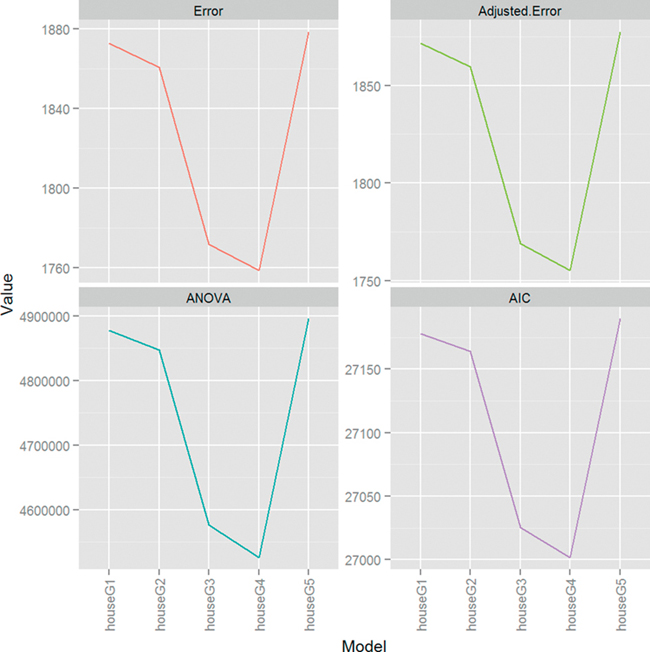
Figure 18.8 Plots for cross-validation error (raw and adjusted), ANOVA and AIC for housing models. The scales are different, as they should be, but the shapes are identical, indicating that houseG4 truly is the best model.
We now present a general framework (loosely borrowed from cv.glm) for running our own cross-validation on models other than glm. This is not universal and will not work for all models, but gives a general idea for how it should be done. In practice it should be abstracted into smaller parts and made more robust.
> cv.work <- function(fun, k = 5, data,
+ cost = function(y, yhat) mean((y - yhat)^2),
+ response="y", ...)
+ {
+ # generate folds
+ folds <- data.frame(Fold=sample(rep(x=1:k, length.out=nrow(data))),
+ Row=1:nrow(data))
+
+ # start the error at 0
+ error <- 0
+
+ ## loop through each of the folds
+ ## for each fold:
+ ## fit the model on the training data
+ ## predict on the test data
+ ## compute the error and accumulate it
+ for(f in 1:max(folds$Fold))
+ {
+ # rows that are in test set
+ theRows <- folds$Row[folds$Fold == f]
+
+ ## call fun on data[-theRows, ]
+ ## predict on data[theRows, ]
+ mod <- fun(data=data[-theRows, ], ...)
+ pred <- predict(mod, data[theRows, ])
+
+ # add new error weighted by the number of rows in this fold
+ error <- error +
+ cost(data[theRows, response], pred) *
+ (length(theRows)/nrow(data))
+ }
+
+ return(error)
+ }
Applying that function to the various housing models we get their cross-validation errors.
> cv1 <- cv.work(fun=lm, k=5, data=housing, response="ValuePerSqFt",
+ formula=ValuePerSqFt ~ Units + SqFt + Boro)
> cv2 <- cv.work(fun=lm, k=5, data=housing, response="ValuePerSqFt",
+ formula=ValuePerSqFt ~ Units * SqFt + Boro)
> cv3 <- cv.work(fun=lm, k=5, data=housing, response="ValuePerSqFt",
+ formula=ValuePerSqFt ~ Units + SqFt * Boro + Class)
> cv4 <- cv.work(fun=lm, k=5, data=housing, response="ValuePerSqFt",
+ formula=ValuePerSqFt ~ Units + SqFt * Boro + SqFt*Class)
> cv5 <- cv.work(fun=lm, k=5, data=housing, response="ValuePerSqFt",
+ formula=ValuePerSqFt ~ Boro + Class)
> cvResults <- data.frame(Model=sprintf("house%s", 1:5),
+ Error=c(cv1, cv2, cv3, cv4, cv5))
> cvResults
Model Error
1 house1 1875.582
2 house2 1859.388
3 house3 1766.066
4 house4 1764.343
5 house5 1880.926
This gives very similar results to cv.glm and again shows that the fourth parameterization is still the best. These measures do not always agree so nicely but it is great when they do.
18.4. Bootstrap
Sometimes, for one reason or another, there is not a good analytic solution to a problem and another tactic is needed. This is especially true for measuring uncertainty for confidence intervals. To overcome this, Bradley Efron introduced the bootstrap in 1979. Since then the bootstrap has grown to revolutionize modern statistics and is indispensable.
The idea is that we start with n rows of data. Some statistic (whether a mean, regression or some arbitrary function) is applied to the data. Then the data are sampled, creating a new dataset. This new set still has n rows except that there are repeats and other rows are entirely missing. The statistic is applied to this new dataset. The process is repeated R times (typically around 1,200), which generates an entire distribution for the statistic. This distribution can then be used to find the mean and confidence interval (typically 95%) for the statistic.
The boot package is a very robust set of tools for making the bootstrap easy to compute. Some care is needed when setting up the function call, but that can be handled easily enough.
Starting with a simple example, we analyze the batting average of Major League Baseball as a whole since 1990. The baseball data have information such as at bats (ab) and hits (h).
> require(plyr)
> baseball <- baseball[baseball$year >= 1990, ]
> head(baseball)
id year stint team lg g ab r h X2b X3b hr rbi sb
67412 alomasa02 1990 1 CLE AL 132 445 60 129 26 2 9 66 4
67414 anderbr01 1990 1 BAL AL 89 234 24 54 5 2 3 24 15
67422 baergca01 1990 1 CLE AL 108 312 46 81 17 2 7 47 0
67424 baineha01 1990 1 TEX AL 103 321 41 93 10 1 13 44 0
67425 baineha01 1990 2 OAK AL 32 94 11 25 5 0 3 21 0
67442 bergmda01 1990 1 DET AL 100 205 21 57 10 1 2 26 3
cs bb so ibb hbp sh sf gidp OBP
67412 1 25 46 2 2 5 6 10 0.3263598
67414 2 31 46 2 5 4 5 4 0.3272727
67422 2 16 57 2 4 1 5 4 0.2997033
67424 1 47 63 9 0 0 3 13 0.3773585
67425 2 20 17 1 0 0 4 4 0.3813559
67442 2 33 17 3 0 1 2 7 0.3750000
The proper way to compute the batting average is to divide total hits by total at bats. This means we cannot simply run mean(h/ab) and sd(h/ab) to get the mean and standard deviation. Rather, the batting average is calculated as sum(h)/sum(ab) and its standard deviation is not easily calculated. This problem is a great candidate for using the bootstrap.
We calculate the overall batting average with the original data. Then we sample n rows with replacement and calculate the batting average again. We do this repeatedly until a distribution is formed. Rather that doing this manually, though, we use boot.
The first argument to boot is the data. The second argument is the function that is to be computed on the data. This function must take at least two arguments (unless sim="parametric" in which case only the first argument is necessary). The first is the original data and the second is a vector of indices, frequencies or weights. Additional named arguments can be passed into the function from boot.
> ## build a function for calculating batting average
> # data is the data
> # boot will pass varying sets of indices
> # some rows will be represented multiple times in a single pass
> # other rows will not be represented at all
> # on average about 63% of the rows will be present
> # this funciton is called repeatedly by boot
> bat.avg <- function(data, indices=1:NROW(data), hits="h",
+ at.bats="ab")
+ {
+ sum(data[indices, hits], na.rm=TRUE) /
+ sum(data[indices, at.bats], na.rm=TRUE)
+ }
>
> # test it on the original data
> bat.avg(baseball)
[1] 0.2745988
>
> # bootstrap it
> # using the baseball data, call bat.avg 1,200 times
> # pass indices to the function
> avgBoot <- boot(data=baseball, statistic=bat.avg, R=1200, stype="i")
>
> # print original measure and estimates of bias and standard error
> avgBoot
ORDINARY NONPARAMETRIC BOOTSTRAP
Call:
boot(data = baseball, statistic = bat.avg, R = 1200, stype = "i")
Bootstrap Statistics :
original bias std. error
t1* 0.2745988 1.071011e-05 0.0006843765
> # print the confidence interval
> boot.ci(avgBoot, conf=.95, type="norm")
BOOTSTRAP CONFIDENCE INTERVAL CALCULATIONS
Based on 1200 bootstrap replicates
CALL :
boot.ci(boot.out = avgBoot, conf = 0.95, type = "norm")
Intervals :
Level Normal
95% ( 0.2732, 0.2759 )
Calculations and Intervals on Original Scale
Visualizing the distribution is as simple as plotting a histogram of the replicate results. Figure 18.9 shows the histogram for the batting average with vertical lines two standard errors on either side of the original estimate. These mark the (roughly) 95% confidence interval.
> ggplot() +
+ geom_histogram(aes(x=avgBoot$t), fill="grey", color="grey") +
+ geom_vline(xintercept=avgBoot$t0 + c(-1, 1)*2*sqrt(var(avgBoot$t)),
+ linetype=2)
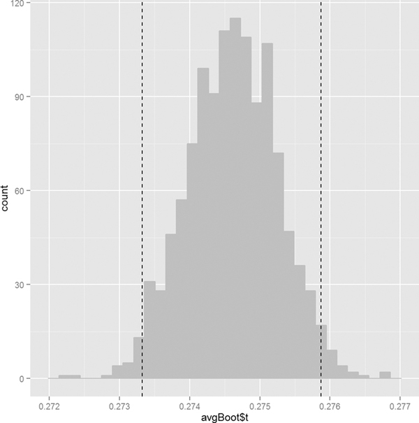
Figure 18.9 Histogram of the batting average bootstrap. The vertical lines are two standard errors from the original estimate in each direction. They make up the bootstrapped 95% confidence interval.
The bootstrap is an incredibly powerful tool that holds a great deal of promise. The boot package offers far more than what we have shown here, including the ability to bootstrap time series and censored data. The beautiful thing about the bootstrap is its near universal applicability. It can be used in just about any situation where an analytical solution is impractical or impossible. There are some instances where the bootstrap is inappropriate, such as for measuring uncertainty of biased estimators like those from the lasso, although such limitations are rare.
18.5. Stepwise Variable Selection
A common, though becoming increasingly discouraged, way to select variables for a model is stepwise selection. This is the process of iteratively adding and removing variables from a model and testing the model at each step, usually using AIC.
The step function iterates through possible models. The scope argument specifies a lower and upper bound on possible models. The direction argument specifies whether variables are just added into the model, just subtracted from the model or added and subtracted as necessary. When run, step prints out all the iterations it has taken to arrive at what it considers the optimal model.
> # the lowest model is the null model, basically the straight average
> nullModel <- lm(ValuePerSqFt ~ 1, data=housing)
> # the largest model we will accept
> fullModel <- lm(ValuePerSqFt ~ Units + SqFt*Boro + Boro*Class,
+ data=housing)
> # try different models
> # start with nullModel
> # do not go above fullModel
> # work in both directions
> houseStep <- step(nullModel,
+ scope=list(lower=nullModel, upper=fullModel),
+ direction="both")
Start: AIC=22151.56
ValuePerSqFt ~ 1
Df Sum of Sq RSS AIC
+ Boro 4 7160206 5137931 19873
+ SqFt 1 1310379 10987758 21858
+ Class 3 1264662 11033475 21873
+ Units 1 778093 11520044 21982
<none> 12298137 22152
Step: AIC=19872.83
ValuePerSqFt ~ Boro
Df Sum of Sq RSS AIC
+ Class 3 242301 4895630 19752
+ SqFt 1 185635 4952296 19778
+ Units 1 83948 5053983 19832
<none> 5137931 19873
- Boro 4 7160206 12298137 22152
Step: AIC=19752.26
ValuePerSqFt ~ Boro + Class
Df Sum of Sq RSS AIC
+ SqFt 1 182170 4713460 19655
+ Units 1 100323 4795308 19700
+ Boro:Class 9 111838 4783792 19710
<none> 4895630 19752
- Class 3 242301 5137931 19873
- Boro 4 6137845 11033475 21873
Step: AIC=19654.91
ValuePerSqFt ~ Boro + Class + SqFt
Df Sum of Sq RSS AIC
+ SqFt:Boro 4 113219 4600241 19599
+ Boro:Class 9 94590 4618870 19620
+ Units 1 37078 4676382 19636
<none> 4713460 19655
- SqFt 1 182170 4895630 19752
- Class 3 238836 4952296 19778
- Boro 4 5480928 10194388 21668
Step: AIC=19599.21
ValuePerSqFt ~ Boro + Class + SqFt + Boro:SqFt
Df Sum of Sq RSS AIC
+ Boro:Class 9 68660 4531581 19578
+ Units 1 23472 4576769 19588
<none> 4600241 19599
- Boro:SqFt 4 113219 4713460 19655
- Class 3 258642 4858883 19737
Step: AIC=19577.81
ValuePerSqFt ~ Boro + Class + SqFt + Boro:SqFt + Boro:Class
Df Sum of Sq RSS AIC
+ Units 1 20131 4511450 19568
<none> 4531581 19578
- Boro:Class 9 68660 4600241 19599
- Boro:SqFt 4 87289 4618870 19620
Step: AIC=19568.14
ValuePerSqFt ~ Boro + Class + SqFt + Units + Boro:SqFt + Boro:Class
Df Sum of Sq RSS AIC
<none> 4511450 19568
- Units 1 20131 4531581 19578
- Boro:Class 9 65319 4576769 19588
- Boro:SqFt 4 75955 4587405 19604
> # reveal the chosen model
> houseStep
Call:
lm(formula = ValuePerSqFt ~ Boro + Class + SqFt + Units + Boro:SqFt +
Boro:Class, data = housing)
Coefficients:
(Intercept)
4.848e+01
BoroBrooklyn
2.655e+01
BoroManhattan
8.672e+01
BoroQueens
1.999e+01
BoroStaten Island
-1.132e+01
ClassR4-CONDOMINIUM
6.586e+00
ClassR9-CONDOMINIUM
4.553e+00
ClassRR-CONDOMINIUM
8.130e+00
SqFt
1.373e-05
Units
-8.296e-02
BoroBrooklyn:SqFt
3.798e-05
BoroManhattan:SqFt
1.594e-04
BoroQueens:SqFt
2.753e-06
BoroStaten Island:SqFt
4.362e-05
BoroBrooklyn:ClassR4-CONDOMINIUM
1.933e+00
BoroManhattan:ClassR4-CONDOMINIUM
3.436e+01
BoroQueens:ClassR4-CONDOMINIUM
1.274e+01
BoroStaten Island:ClassR4-CONDOMINIUM
NA
BoroBrooklyn:ClassR9-CONDOMINIUM
-3.440e+00
BoroManhattan:ClassR9-CONDOMINIUM
1.497e+01
BoroQueens:ClassR9-CONDOMINIUM
-9.967e+00
BoroStaten Island:ClassR9-CONDOMINIUM
NA
BoroBrooklyn:ClassRR-CONDOMINIUM
-2.901e+01
BoroManhattan:ClassRR-CONDOMINIUM
-6.850e+00
BoroQueens:ClassRR-CONDOMINIUM
2.989e+01
BoroStaten Island:ClassRR-CONDOMINIUM
NA
Ultimately, step decided that fullModel was optimal with the lowest AIC. While this works, it is a bit of a brute force method and has its own theoretical problems. Lasso regression arguably does a better job of variable selection and is discussed in Section 19.1.
18.6. Conclusion
Determining the quality of a model is an important step in the model-building process. This can take the form of traditional tests of fit such as ANOVA or more modern techniques like cross-validation. The bootstrap is another means of determining model uncertainty, especially for models where confidence intervals are impractical to calculate. These can all be shaped by helping select which variables are included in a model and which are excluded.