
Chapter 19. Regularization and Shrinkage
In today’s era of high dimensional (many variables) data, methods are needed to prevent overfitting. Traditionally, this has been done with variable selection, as described in Chapter 18, although with a large number of variables that can become computationally prohibitive. These methods can take a number of forms; we focus on regularization and shrinkage. For these we will use glmnet from the glmnet package and bayesglm from the arm package.
19.1. Elastic Net
One of the most exciting algorithms to be developed in the past five years is the Elastic Net, which is a dynamic blending of lasso and ridge regression. The lasso uses an L1 penalty to perform variable selection and dimension reduction, while the ridge uses an L2 penalty to shrink the coefficients for more stable predictions. The formula for the Elastic Net is
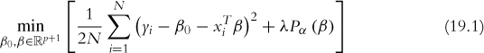
where
where λ is a complexity parameter controlling the amount of shrinkage (0 is no penalty and ∞ is complete penalty) and α regulates how much of the solution is ridge versus lasso with α = 0 being complete ridge and α = 1 being complete lasso. Γ, not seen here, is a vector of penalty factors—one value per variable—that multiplies λ for fine tuning of the penalty applied to each variable; again 0 is no penalty and ∞ is complete penalty.
A fairly new package (this is a relatively new algorithm) is glmnet, which fits generalized linear models with the Elastic Net. It is written by Trevor Hastie, Robert Tibshirani and Jerome Friedman from Stanford University who also published the landmark papers on the Elastic Net.
Because it is designed for speed and larger, sparser data, glmnet requires a little more effort to use than most other modeling functions in R. Where functions like lm and glm take a formula to specify the model, glmnet requires a matrix of predictors (excluding an intercept, as it is added automatically) and a response matrix.
Even though it is not incredibly high dimensional, we will look at the American Community Survey (ACS) data for New York State. We will throw every possible predictor into the model and see which are selected.
> acs <- read.table("http://jaredlander.com/data/acs_ny.csv", sep = ",",
+ header = TRUE, stringsAsFactors = FALSE)
Because glmnet requires a predictor matrix, it will be good to have a convenient way of building that matrix. This can be done simply enough using model.matrix, which at its most basic takes in a formula and a data.frame and returns a design matrix. As an example we create some fake data and run model.matrix on it.
> # build a data.frame where the first three columns are numeric
> testFrame <-
+ data.frame(First=sample(1:10, 20, replace=TRUE),
+ Second=sample(1:20, 20, replace=TRUE),
+ Third=sample(1:10, 20, replace=TRUE),
+ Fourth=factor(rep(c("Alice", "Bob", "Charlie", "David"),
+ 5)),
+ Fifth=ordered(rep(c("Edward", "Frank", "Georgia",
+ "Hank", "Isaac"), 4)),
+ Sixth=rep(c("a", "b"), 10), stringsAsFactors=F)
> head(testFrame)
First Second Third Fourth Fifth Sixth
1 3 8 6 Alice Edward a
2 3 16 4 Bob Frank b
3 9 14 6 Charlie Georgia a
4 9 2 2 David Hank b
5 5 17 6 Alice Isaac a
6 6 3 4 Bob Edward b
>
> head(model.matrix(First ~ Second + Fourth + Fifth, testFrame))
(Intercept) Second FourthBob FourthCharlie FourthDavid Fifth.L
1 1 8 0 0 0 -0.6324555
2 1 16 1 0 0 -0.3162278
3 1 14 0 1 0 0.0000000
4 1 2 0 0 1 0.3162278
5 1 17 0 0 0 0.6324555
6 1 3 1 0 0 -0.6324555
Fifth.Q Fifth.C Fifth^4
1 0.5345225 -3.162278e-01 0.1195229
2 -0.2672612 6.324555e-01 -0.4780914
3 -0.5345225 -4.095972e-16 0.7171372
4 -0.2672612 -6.324555e-01 -0.4780914
5 0.5345225 3.162278e-01 0.1195229
6 0.5345225 -3.162278e-01 0.1195229
This works very well and is simple, but first there are a few things to notice. As expected, Fourth gets converted into indicator variables with one less column than levels in Fourth. Initially, the parameterization of Fifth might seem odd, as there is one less column than there are levels, but their values are not just 1s and 0s. This is because Fifth is an ordered factor where one level is greater or less than another level.
Not creating an indicator variable for the base level of a factor is essential for most linear models to avoid multicollinearity.1 However, it is generally considered undesirable for the predictor matrix to be designed this way for the Elastic Net. It is possible to have model.matrix return indicator variables for all levels of a factor, although doing so can take some creative coding.2 To make the process easier we incorporated a solution in the build.x function in the useful package.
1. This is a characteristic of a matrix in linear algebra where the columns are not linearly independent. While this is an important concept, we do not need to concern ourselves with it much in the context of this book.
2. The difficulty is evidenced in this Stack Overflow question asked by us: http://stackoverflow.com/questions/4560459/all-levels-of-a-factor-in-a-model-matrix-in-r/15400119
> require(useful)
> # always use all levels
> head(build.x(First ~ Second + Fourth + Fifth, testFrame,
+ contrasts=FALSE))
(Intercept) Second FourthAlice FourthBob FourthCharlie FourthDavid
1 1 8 1 0 0 0
2 1 16 0 1 0 0
3 1 14 0 0 1 0
4 1 2 0 0 0 1
5 1 17 1 0 0 0
6 1 3 0 1 0 0
FifthEdward FifthFrank FifthGeorgia FifthHank FifthIsaac
1 1 0 0 0 0
2 0 1 0 0 0
3 0 0 1 0 0
4 0 0 0 1 0
5 0 0 0 0 1
6 1 0 0 0 0
> # just use all levels for Fourth
> head(build.x(First ~ Second + Fourth + Fifth, testFrame,
+ contrasts=c(Fourth=FALSE, Fifth=TRUE)))
(Intercept) Second FourthAlice FourthBob FourthCharlie FourthDavid
1 1 8 1 0 0 0
2 1 16 0 1 0 0
3 1 14 0 0 1 0
4 1 2 0 0 0 1
5 1 17 1 0 0 0
6 1 3 0 1 0 0
Fifth.L Fifth.Q Fifth.C Fifth^4
1 -0.6324555 0.5345225 -3.162278e-01 0.1195229
2 -0.3162278 -0.2672612 6.324555e-01 -0.4780914
3 0.0000000 -0.5345225 -4.095972e-16 0.7171372
4 0.3162278 -0.2672612 -6.324555e-01 -0.4780914
5 0.6324555 0.5345225 3.162278e-01 0.1195229
6 -0.6324555 0.5345225 -3.162278e-01 0.1195229
Using build.x appropriately on acs builds a nice predictor matrix for use in glmnet. We control the desired matrix by using a formula for our model specification just like we would in lm, interactions and all.
> # make a binary Income variable for building a logistic regression
> acs$Income <- with(acs, FamilyIncome >= 150000)
>
> head(acs)
Acres FamilyIncome FamilyType NumBedrooms NumChildren NumPeople
1 1-10 150 Married 4 1 3
2 1-10 180 Female Head 3 2 4
3 1-10 280 Female Head 4 0 2
4 1-10 330 Female Head 2 1 2
5 1-10 330 Male Head 3 1 2
6 1-10 480 Male Head 0 3 4
NumRooms NumUnits NumVehicles NumWorkers OwnRent
1 9 Single detached 1 0 Mortgage
2 6 Single detached 2 0 Rented
3 8 Single detached 3 1 Mortgage
4 4 Single detached 1 0 Rented
5 5 Single attached 1 0 Mortgage
6 1 Single detached 0 0 Rented
YearBuilt HouseCosts ElectricBill FoodStamp HeatingFuel Insurance
1 1950-1959 1800 90 No Gas 2500
2 Before 1939 850 90 No Oil 0
3 2000-2004 2600 260 No Oil 6600
4 1950-1959 1800 140 No Oil 0
5 Before 1939 860 150 No Gas 660
6 Before 1939 700 140 No Gas 0
Language Income
1 English FALSE
2 English FALSE
3 Other European FALSE
4 English FALSE
5 Spanish FALSE
6 English FALSE
>
> # build predictor matrix
> # do not include the intercept as glmnet will add that automatically
> acsX <- build.x(Income ~ NumBedrooms + NumChildren + NumPeople +
+ NumRooms + NumUnits + NumVehicles + NumWorkers +
+ OwnRent + YearBuilt + ElectricBill + FoodStamp +
+ HeatingFuel + Insurance + Language - 1,
+ data=acs, contrasts=FALSE)
>
> # check class and dimensions
> class(acsX)
[1] "matrix"
> dim(acsX)
[1] 22745 44
>
> # view the top left and top right of the data
> topleft(acsX, c=6)
NumBedrooms NumChildren NumPeople NumRooms NumUnitsMobile home
1 4 1 3 9 0
2 3 2 4 6 0
3 4 0 2 8 0
4 2 1 2 4 0
5 3 1 2 5 0
NumUnitsSingle attached
1 0
2 0
3 0
4 0
5 1
> topright(acsX, c=6)
Insurance LanguageAsian Pacific LanguageEnglish LanguageOther
1 2500 0 1 0
2 0 0 1 0
3 6600 0 0 0
4 0 0 1 0
5 660 0 0 0
LanguageOther European LanguageSpanish
1 0 0
2 0 0
3 1 0
4 0 0
5 0 1
>
> # build response predictor
> acsY <- build.y(Income ~ NumBedrooms + NumChildren + NumPeople +
+ NumRooms + NumUnits + NumVehicles + NumWorkers +
+ OwnRent + YearBuilt + ElectricBill + FoodStamp +
+ HeatingFuel + Insurance + Language - 1, data=acs)
>
> head(acsY)
[1] FALSE FALSE FALSE FALSE FALSE FALSE
> tail(acsY)
[1] TRUE TRUE TRUE TRUE TRUE TRUE
Now that the data are properly stored we can run glmnet. As seen in Equation 19.1, λ controls the amount of shrinkage. By default glmnet fits the regularization path on 100 different values of λ. The decision of which is best then falls upon the user with cross-validation being a good measure. Fortunately, the glmnet package has a function, cv.glmnet, that computes the cross-validation automatically. By default α = 1, meaning only the lasso is calculated. Selecting the best α requires an additional layer of cross-validation.
> require(glmnet)
> set.seed(1863561)
> # run the cross-validated glmnet
> acsCV1 <- cv.glmnet(x = acsX, y = acsY, family = "binomial", nfold = 5)
The most important information returned from cv.glmnet are the cross-validation error and which value of λ minimizes the cross-validation error. Additionally, it also returns the largest value of λ with a cross-validation error that is within one standard error of the minimum. Theory suggests that the simpler model, even though it is slightly less accurate, should be preferred due to its parsimony. The cross-validation errors for differing values of λ are seen in Figure 19.1. The top row of numbers indicates how many variables (factor levels are counted as individual variables) are in the model for a given value of log(λ).

Figure 19.1 Cross-validation curve for the glmnet fitted on the American Community Survey data. The top row of numbers indicates how many variables (factor levels are counted as individual variables) are in the model for a given value of log(λ). The dots represent the cross-validation error at that point and the vertical lines are the confidence interval for the error. The leftmost vertical line indicates the value of λ where the error is minimized and the rightmost vertical line is the next largest value of λ error that is within one standard error of the minimum.
> acsCV1$lambda.min
[1] 0.0005258299
> acsCV1$lambda.1se
[1] 0.006482677
> plot(acsCV1)
Extracting the coefficients is done as with any other model, by using coef, except that a specific level of λ should be specified; otherwise, the entire path is returned. Dots represent variables that were not selected.
> coef(acsCV1, s = "lambda.1se")
45 x 1 sparse Matrix of class "dgCMatrix"
1
(Intercept) -5.0552170103
NumBedrooms 0.0542621380
NumChildren .
NumPeople .
NumRooms 0.1102021934
NumUnitsMobile home -0.8960712560
NumUnitsSingle attached .
NumUnitsSingle detached .
NumVehicles 0.1283171343
NumWorkers 0.4806697219
OwnRentMortgage .
OwnRentOutright 0.2574766773
OwnRentRented -0.1790627645
YearBuilt15 .
YearBuilt1940-1949 -0.0253908040
YearBuilt1950-1959 .
YearBuilt1960-1969 .
YearBuilt1970-1979 -0.0063336086
YearBuilt1980-1989 0.0147761442
YearBuilt1990-1999 .
YearBuilt2000-2004 .
YearBuilt2005 .
YearBuilt2006 .
YearBuilt2007 .
YearBuilt2008 .
YearBuilt2009 .
YearBuilt2010 .
YearBuiltBefore 1939 -0.1829643904
ElectricBill 0.0018200312
FoodStampNo 0.7071289660
FoodStampYes .
HeatingFuelCoal -0.2635263281
HeatingFuelElectricity .
HeatingFuelGas .
HeatingFuelNone .
HeatingFuelOil .
HeatingFuelOther .
HeatingFuelSolar .
HeatingFuelWood -0.7454315355
Insurance 0.0004973315
LanguageAsian Pacific 0.3606176925
LanguageEnglish .
LanguageOther .
LanguageOther European 0.0389641675
LanguageSpanish .
It might seem weird that some levels of a factor were selected and others were not, but it ultimately makes sense because the lasso eliminates variables that are highly correlated with each other.
Another thing to notice is that there are no standard errors and hence no confidence intervals for the coefficients. The same is true of any predictions made from a glmnet model. This is due to the theoretical properties of the lasso and ridge, and is an open problem. Recent advancements have led to the ability to perform significance tests on lasso regressions, although the existing R package requires that the model be fitted using the lars package, not glmnet, at least until the research extends the testing ability to cover the Elastic Net as well.
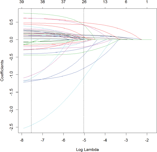
Visualizing where variables enter the model along the λ path can be illuminating and is seen in Figure 19.2.
> # plot the path
> plot(acsCV1$glmnet.fit, xvar = "lambda")
> # add in vertical lines for the optimal values of lambda
> abline(v = log(c(acsCV1$lambda.min, acsCV1$lambda.1se)), lty = 2)

Figure 19.2 Coefficient profile plot of the glmnet model fitted on the ACS data. Each line represents a coefficient’s value at different values of λ. The leftmost vertical line indicates the value of λ where the error is minimized and the rightmost vertical line is the next largest value of λ error that is within one standard error of the minimum.
Setting α to 0 causes the results to be from the ridge. In this case, every variable is kept in the model but is just shrunk closer to 0. Figure 19.3, on page 283, shows the cross-validation curve. Notice in Figure 19.4, on page 284, that for every value of λ there are still all the variables, just at different sizes.
> # fit the ridge model
> set.seed(71623)
> acsCV2 <- cv.glmnet(x = acsX, y = acsY, family = "binomial", nfold = 5,
+ alpha = 0)
> # look at the lambda values
> acsCV2$lambda.min
[1] 0.01272576
> acsCV2$lambda.1se
[1] 0.04681018
>
> # look at the coefficients
> coef(acsCV2, s = "lambda.1se")
45 x 1 sparse Matrix of class "dgCMatrix"
1
(Intercept) -4.8197810188
NumBedrooms 0.1027963294
NumChildren 0.0308893447
NumPeople -0.0203037177
NumRooms 0.0918136969
NumUnitsMobile home -0.8470874369
NumUnitsSingle attached 0.1714879712
NumUnitsSingle detached 0.0841095530
NumVehicles 0.1583881396
NumWorkers 0.3811651456
OwnRentMortgage 0.1985621193
OwnRentOutright 0.6480126218
OwnRentRented -0.2548147427
YearBuilt15 -0.6828640400
YearBuilt1940-1949 -0.1082928305
YearBuilt1950-1959 0.0602009151
YearBuilt1960-1969 0.0081133932
YearBuilt1970-1979 -0.0816541923
YearBuilt1980-1989 0.1593567244
YearBuilt1990-1999 0.1218212609
YearBuilt2000-2004 0.1768690849
YearBuilt2005 0.2923210334
YearBuilt2006 0.2309044444
YearBuilt2007 0.3765019705
YearBuilt2008 -0.0648999685
YearBuilt2009 0.2382560699
YearBuilt2010 0.3804282473
YearBuiltBefore 1939 -0.1648659906
ElectricBill 0.0018576432
FoodStampNo 0.3886474609
FoodStampYes -0.3886013004
HeatingFuelCoal -0.7005075763
HeatingFuelElectricity -0.1370927269
HeatingFuelGas 0.0873505398
HeatingFuelNone -0.5983944720
HeatingFuelOil 0.1241958119
HeatingFuelOther -0.1872564710
HeatingFuelSolar -0.0870480957
HeatingFuelWood -0.6699727752
Insurance 0.0003881588
LanguageAsian Pacific 0.3982023046
LanguageEnglish -0.0851389569
LanguageOther 0.1804675114
LanguageOther European 0.0964194255
LanguageSpanish -0.1274688978
>
> # plot the cross-validation error path
> plot(acsCV2)
> # plot the coefficient path
> plot(acsCV2$glmnet.fit, xvar = "lambda")
> abline(v = log(c(acsCV2$lambda.min, acsCV2$lambda.1se)), lty = 2)


Finding the optimal value of α requires an additional layer of cross-validation, and unfortunately glmnet does not do that automatically. This will require us to run cv.glmnet at various levels of α, which will take a fairly large chunk of time if performed sequentially, making this a good time to use parallelization. The most straightforward way to run code in parallel is to the use the parallel, doParallel and foreach packages.
> require(parallel)
Loading required package: parallel
> require(doParallel)
Loading required package: doParallel
Loading required package: foreach
Loading required package: iterators
First, we build some helper objects to speed along the process. When a two-layered cross-validation is run, an observation should fall in the same fold each time, so we build a vector specifying fold membership. We also specify the sequence of α values that foreach will loop over. It is generally considered better to lean toward the lasso rather than the ridge, so we consider only α values greater than 0.5.
> # set the seed for repeatability of random results
> set.seed(2834673)
>
> # create folds, we want observations to be in the same fold each time
> # it is run
> theFolds <- sample(rep(x = 1:5, length.out = nrow(acsX)))
>
> # make sequence of alpha values
> alphas <- seq(from = 0.5, to = 1, by = 0.05)
Before running a parallel job, a cluster (even on a single machine) must be started and registered with makeCluster and registerDoParallel. After the job is done the cluster should be stopped with stopCluster. Setting .errorhandling to ''remove'' means that if an error occurs, that iteration will be skipped. Setting .inorder to FALSE means that the order of combining the results does not matter and they can be combined whenever returned, which yields significant speed improvements. Because we are using the default combination function, list, which takes multiple arguments at once, we can speed up the process by setting .multicombine to TRUE. We specify in .packages that glmnet should be loaded on each of the workers, again leading to performance improvements. The operator %dopar% tells foreach to work in parallel. Parallel computing can be dependent on the environment, so we explicitly load some variables into the foreach environment using .export, namely, acsX, acsY, alphas and theFolds.
> # set the seed for repeatability of random results
> set.seed(5127151)
>
> # start a cluster with two workers
> cl <- makeCluster(2)
> # register the workers
> registerDoParallel(cl)
>
> # keep track of timing
> before <- Sys.time()
>
> # build foreach loop to run in parallel
> ## several arguments
> acsDouble <- foreach(i=1:length(alphas), .errorhandling="remove",
+ .inorder=FALSE, .multicombine=TRUE,
+ .export=c("acsX", "acsY", "alphas", "theFolds"),
+ .packages="glmnet") %dopar%
+ {
+ print(alphas[i])
+ cv.glmnet(x=acsX, y=acsY, family="binomial", nfolds=5,
+ foldid=theFolds, alpha=alphas[i])
+ }
>
> # stop timing
> after <- Sys.time()
>
> # make sure to stop the cluster when done
> stopCluster(cl)
>
> # time difference
> # this will depend on speed, memory & number of cores of the machine
> after - before
Time difference of 1.443783 mins
The results in acsDouble should be a list with 11 instances of cv.glmnet objects. We can use sapply to check the class of each element of the list.
> sapply(acsDouble, class)
[1] "cv.glmnet" "cv.glmnet" "cv.glmnet" "cv.glmnet" "cv.glmnet"
[6] "cv.glmnet" "cv.glmnet" "cv.glmnet" "cv.glmnet" "cv.glmnet"
[11] "cv.glmnet"
The goal is to find the best combination of λ and α, so we need to build some code to extract the cross-validation error (including the confidence interval) and λ from each element of the list.
> # function for extracting info from cv.glmnet object
> extractGlmnetInfo <- function(object)
+ {
+ # find lambdas
+ lambdaMin <- object$lambda.min
+ lambda1se <- object$lambda.1se
+
+ # figure out where those lambdas fall in the path
+ whichMin <- which(object$lambda == lambdaMin)
+ which1se <- which(object$lambda == lambda1se)
+
+ # build a one line data.frame with each of the selected lambdas and
+ # its corresponding error figures
+ data.frame(lambda.min=lambdaMin, error.min=object$cvm[whichMin],
+ lambda.1se=lambda1se, error.1se=object$cvm[which1se])
+ }
>
> # apply that function to each element of the list
> # combine it all into a data.frame
> alphaInfo <- Reduce(rbind, lapply(acsDouble, extractGlmnetInfo))
>
> # could also be done with ldply from plyr
> alphaInfo2 <- plyr::ldply(acsDouble, extractGlmnetInfo)
> identical(alphaInfo, alphaInfo2)
[1] TRUE
>
> # make a column listing the alphas
> alphaInfo$Alpha <- alphas
> alphaInfo
lambda.min error.min lambda.1se error.1se Alpha
1 0.0009582333 0.8220267 0.008142621 0.8275331 0.50
2 0.0009560545 0.8220226 0.007402382 0.8273936 0.55
3 0.0008763832 0.8220197 0.006785517 0.8272771 0.60
4 0.0008089692 0.8220184 0.006263554 0.8271786 0.65
5 0.0008244253 0.8220168 0.005816158 0.8270917 0.70
6 0.0007694636 0.8220151 0.005428414 0.8270161 0.75
7 0.0007213721 0.8220139 0.005585323 0.8276118 0.80
8 0.0006789385 0.8220130 0.005256774 0.8275519 0.85
9 0.0006412197 0.8220123 0.004964731 0.8274993 0.90
10 0.0006074713 0.8220128 0.004703430 0.8274524 0.95
11 0.0005770977 0.8220125 0.004468258 0.8274120 1.00
Now that we have this nice, unintelligible set of numbers, we should plot it to easily pick out the best combination of α and λ, which is where the plot shows minimum error. Figure 19.5 indicates that by using the one standard error methodology, the optimal α and λ are 0.75 and 0.0054284, respectively.
> ## prepare the data.frame for plotting multiple pieces of information
> require(reshape2)
> require(stringr)
>
> # melt the data into long format
> alphaMelt <- melt(alphaInfo, id.vars="Alpha", value.name="Value",
+ variable.name="Measure")
> alphaMelt$Type <- str_extract(string=alphaMelt$Measure,
+ pattern="(min)|(1se)")
>
> # some housekeeping
> alphaMelt$Measure <- str_replace(string=alphaMelt$Measure,
+ pattern="\.(min|1se)",
+ replacement="")
> alphaCast <- dcast(alphaMelt, Alpha + Type ~ Measure,
+ value.var="Value")
>
> ggplot(alphaCast, aes(x=Alpha, y=error)) +
+ geom_line(aes(group=Type)) +
+ facet_wrap(~Type, scales="free_y", ncol=1) +
+ geom_point(aes(size=lambda))

Figure 19.5 Plot of α versus error for glmnet cross-validation on the ACS data. The lower the error the better. The size of the dot represents the value of lambda. The top pane shows the error using the one standard error methodology (0.0054) and the bottom pane shows the error by selecting the λ (6e-04) that minimizes the error. In the top pane the error is minimized for an α of 0.75 and in the bottom pane the optimal α is 0.9.
Now that we have found the optimal value of α (0.75), we refit the model and check the results.
> set.seed(5127151)
> acsCV3 <- cv.glmnet(x = acsX, y = acsY, family = "binomial", nfold = 5,
+ alpha = alphaInfo$Alpha[which.min(alphaInfo$error.1se)])
After fitting the model we check the diagnostic plots shown in Figures 19.6 and 19.7.

> plot(acsCV3)
> plot(acsCV3$glmnet.fit, xvar = "lambda")
> abline(v = log(c(acsCV3$lambda.min, acsCV3$lambda.1se)), lty = 2)
Viewing the coefficient plot for a glmnet object is not yet implemented in coefplot, so we build it manually. Figure 19.8 shows that the number of workers in the family and not being on foodstamps are the strongest indicators of having high income, and using coal heat and living in a mobile home are the strongest indicators of having low income. There are no standard errors because glmnet does not calculate them.
> theCoef <- as.matrix(coef(acsCV3, s = "lambda.1se"))
> coefDF <- data.frame(Value = theCoef,
+ Coefficient = rownames(theCoef))
> coefDF <- coefDF[nonzeroCoef(coef(acsCV3, s = "lambda.1se")), ]
> ggplot(coefDF, aes(x = X1, y = reorder(Coefficient, X1))) +
+ geom_vline(xintercept = 0, color = "grey", linetype = 2) +
+ geom_point(color = "blue") + labs(x = "Value",
+ y = "Coefficient", title = "Coefficient Plot")
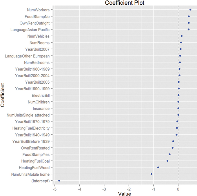
Figure 19.8 Coefficient plot for glmnet on ACS data. This shows that the number of workers in the family and not being on foodstamps are the strongest indicators of having high income, and using coal heat and living in a mobile home are the strongest indicators of having low income. There are no standard errors because glmnet does not calculate them.
19.2. Bayesian Shrinkage
For Bayesians, shrinkage can come in the form of weakly informative priors.3 This can be particularly useful when a model is built on data that does not have a large enough number of rows for some combinations of the variables. For this example, we blatantly steal an example from Andrew Gelman’s and Jennifer Hill’s book, Data Analysis Using Regression and Multilevel/Hierarchical Models, examining voter preference. The data have been cleaned up and posted at http://jaredlander.com/data/ideo.rdata.
3. From a Bayesian point of view, the penalty terms in the Elastic Net could be considered log-priors as well.
> load("data/ideo.rdata")
> head(ideo)
Year Vote Age Gender Race
1 1948 democrat NA male white
2 1948 republican NA female white
3 1948 democrat NA female white
4 1948 republican NA female white
5 1948 democrat NA male white
6 1948 republican NA female white
Education Income
1 grade school of less (0-8 grades) 34 to 67 percentile
2 high school (12 grades or fewer, incl 96 to 100 percentile
3 high school (12 grades or fewer, incl 68 to 95 percentile
4 some college(13 grades or more,but no 96 to 100 percentile
5 some college(13 grades or more,but no 68 to 95 percentile
6 high school (12 grades or fewer, incl 96 to 100 percentile
Religion
1 protestant
2 protestant
3 catholic (roman catholic)
4 protestant
5 catholic (roman catholic)
6 protestant
To show the need for shrinkage, we fit a separate model for each election year and then display the resulting coefficients for the black level of Race.
> ## fit a bunch of models
> # figure out the years we will be fitting the models on
> theYears <- unique(ideo$Year)
>
> # create an empty list
> # as many elements as years
> # it holds the results
> # preallocating the object makes the code run faster
> results <- vector(mode="list", length=length(theYears))
> # give good names to the list
> names(results) <- theYears
>
> ## loop through the years
> # fit a model on the subset of data for that year
> for(i in theYears)
+ {
+ results[[as.character(i)]] <- glm(Vote ~ Race + Income + Gender +
+ Education,
+ data=ideo, subset=Year==i,
+ family=binomial(link="logit"))
+ }
Now that we have all of these models, we can plot the coefficients with multiplot. Figure 19.9 shows the coefficient for the black level of Race for each model. The result for the model from 1964 is clearly far different from the other models. Figure 19.9 shows standard errors, which threw off the scale so much that we had to restrict the plot window to still see variation in the other points. Fitting a series of models like this and then plotting the coefficients over time has been termed the “secret weapon” by Gelman due to its usefulness and simplicity.

Figure 19.9 Plot showing the coefficient for the black level of Race for each of the models. The coefficient for 1964 has a standard error that is orders of magnitude bigger than for the other years. It is so out of proportion that the plot had to be truncated to still see variation in the other data points.
> require(coefplot)
> # get the coefficient information
> voteInfo <- multiplot(results, coefficients="Raceblack", plot=FALSE)
> head(voteInfo)
Value Coefficient HighInner LowInner HighOuter
1 0.07119541 Raceblack 0.6297813 -0.4873905 1.1883673
2 -1.68490828 Raceblack -1.3175506 -2.0522659 -0.9501930
3 -0.89178359 Raceblack -0.5857195 -1.1978476 -0.2796555
4 -1.07674848 Raceblack -0.7099648 -1.4435322 -0.3431811
5 -16.85751152 Raceblack 382.1171424 -415.8321655 781.0917963
6 -3.65505395 Raceblack -3.0580572 -4.2520507 -2.4610605
LowOuter Model
1 -1.045976 1948
2 -2.419624 1952
3 -1.503912 1956
4 -1.810316 1960
5 -814.806819 1964
6 -4.849047 1968
>
> # plot it restricting the window to (-20, 10)
> multiplot(results, coefficients="Raceblack", secret.weapon=TRUE) +
+ coord_flip(xlim=c(-20, 10))
By comparing the model for 1964 to the other models, we can see that something is clearly wrong with the estimate. To fix this we put a prior on the coefficients in the model. The simplest way to do this is to use Gelman’s bayesglm function in the arm package. By default it sets a Cauchy prior with scale 2.5. Because the arm package namespace interferes with the coefplot namespace, we do not load the package but rather just call the function using the :: operator.
> resultsB <- vector(mode="list", length=length(theYears))
> # give good names to the list
> names(resultsB) <- theYears
>
> ## loop through the years
> ## fit a model on the subset of data for that year
> for(i in theYears)
+ {
+ # fit model with Cauchy priors with a scale of 2.5
+ resultsB[[as.character(i)]] <-
+ arm::bayesglm(Vote ~ Race + Income + Gender + Education,
+ data=ideo[ideo$Year == i, ],
+ family=binomial(link="logit"),
+ prior.scale=2.5, prior.df=1)
+ }
>
> # build the coefficient plot
> multiplot(resultsB, coefficients="Raceblack", secret.weapon=TRUE)
Simply adding Cauchy priors dramatically shrinks both the estimate and the standard error of the coefficient, as seen in Figure 19.10. Remember, the models were fitted independently, meaning that it was simply the prior that did the fix and not information from the other years. It turns out that the survey conducted in 1964 underrepresented black respondents, which led to a highly inaccurate measure.
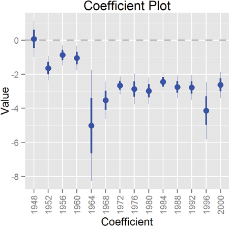
Figure 19.10 Coefficient plot (the secret weapon) for the black level of Race for each of the models with a Cauchy prior. A simple change like adding a prior dramatically changed the point estimate and standard error.
The default prior is a Cauchy with scale 2.5, which is the same as a t distribution with 1 degree of freedom. These arguments, prior.scale and prior.df, can be changed to represent a t distribution with any degrees of freedom. Setting both to infinity (Inf) makes them normal priors, which is identical to running an ordinary glm.
19.3. Conclusion
Regularization and shrinkage play important roles in modern statistics. They help fit models to poorly designed data, and prevent overfitting of complex models. The former is done using Bayesian methods, in this case the simple bayesglm; the latter is done with the lasso, ridge or Elastic Net using glmnet. Both are useful tools to have.