21. The New Sustainable EOQ Formula

The Economic Order Quantity (EOQ) is the amount needed to be ordered to minimize the variable cost. The EOQ formula looks only at the activity on the plant floor or in the distribution area. This chapter takes this formula to a new dimension. It expands the horizon of the EOQ formula to the entire supply chain and into the sustainable age of Green. The EOQ is the amount of inventory purchased that will balance the ordering and holding costs. Inventory is composed of the following parts:

• Raw materials and purchased parts from outside suppliers.

• Components and subassemblies that are awaiting final assembly.

• Work in process, which is all materials or components on the production floor in various stages of production.

• Finished goods, which are the final products waiting for purchase or to be sent to customers.

• Supplies, which are all items that are needed but that are not part of the finished product, such as paper clips, duplicating machine toner, and tools. This also includes the Maintenance Repair and Operations items.

Inventory Management is the process of ensuring that the firm has adequate inventories of all parts and supplies needed within the constraint of minimizing total inventory costs. The total inventory costs are composed of ordering (setup) costs, acquisition costs, holding (carrying) costs, and stock-out costs.

To be Lean and Green, the transportation component must be minimized. The existing EOQ formula is concerned only with the effect of holding and receiving costs. As the order quantity (OQ) increases, a Total Cost (TC) curve hits a minimum where the slope equals zero. After that, the TC slope turns positive and the total costs will start increasing.

Including the freight component along with the holding and receiving costs represents the transportation phase of the supply chain. When decreasing the EOQ to lower inventory cost, the transportation cost must be added to the EOQ equation. As the EOQ increases, the transportation costs decrease due to less-frequent shipping. Holding costs increase but the number of deliveries decreases.

• Inventory is divided into three dollar-volume categories—A, B, and C—with the A parts being the most active (largest dollar volume). The idea is to focus most on the high-annual-dollar volume A inventory items, then to a lesser extent on the B items, and even less on the C items.

• Inventory A items have the highest safety stock to guard against costly stock-outs. This can be performed in a number of ways. These are the variables:

• Q = number of pieces per year.

• EOQ = optimum number of pieces per year.

• D = annual demand in units of inventory items per year.

• S = setup cost or ordering cost for each order in $.

• H = holding or carrying cost per unit, per year, in $.

• d = demand during a demand period.

• F = freight rate.

• P = purchase price or cost of inventory.

• N = number of orders per year which yields .

• LT = the lead time for the vendor.

• RT = the time between reviews of the supplier, called review time.

• Annual setup costs . The ordering cost can also be used for this analysis depending on what is minimized.

• The average inventory is defined as .

• Annual holding costs .

• Optimum inventory is found when the annual setup costs = annual holding costs.

• Where .

• So .

• .

• So the total cost of inventory is minimized when holding costs equal setup costs.

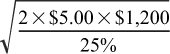
Let’s use the preceding concept to create a graph of the EOQ formula (Figure 21-1), using the following values:

• D = $1,200 annual demand.

• S = the ordering costs are $5.00 per order.

• H = the holding cost of inventory, which is an annualized figure of 25%.

Figure 21-1 shows the simulation of the EOQ formula run for 52 periods. The graph in Figure 21-1 shows the minimum point in the EOQ formula where ordering cost and holding costs cross each other.

Figure 21-1. The graph of the EOQ formula

Note that the point where the holding costs equal the ordering costs is where the EOQ = 219. The calculation is

On the graph, the period at 26 places the EOQ at 220. This is where the HC graph crosses the SC graph, resulting in the lowest total cost.

At this point, it is necessary to introduce the safety stock because the entire order quantity is made up of the forecast plus safety stock minus on-hand and on-order. The order quantity is now ordered in multiples of the EOQ.

In forecasting, the value k measures the amount of safety stock to use. The k is the equivalent of Z in a probability transform. The k value is used with the mean average deviation (MAD), whereas the Z value is used for standard deviation. The k measures the amount of safety stock needed according to the required item service level.

When the system reads a higher k value, it orders more safety stock. With k set for a 98% fill rate for A items and a 90% fill rate for B items and 85% fill rate for C items, this is called forecasting using the service level to determine the ABC analysis. The formula is OQ = d * (LT + RT) + k * (LT + RT)^.7.

• d = the demand for the period.

• OQ = the order quantity.

• LT = the lead time including manufacturing lead time plus transit time and receiving to stock time.

• RT = the review time, which is the time between reviews. This assumes a fixed-period forecasting schedule.

• k = the forecast standard deviation used for determining service level when using MAD.

• The (LT + RT^).7 to the .7 power is used to get the most accurate lead-time variability for MAD.

It is possible to alternatively add extra lead time for A items and decrease the extra lead time for C items, but this does not result in a quantified answer to the service-level goal. It simply allows for adding to improve the service level. There is no guide available to indicate what the improvement will be. Using the k values results in enough measurable performance criteria on which to base the reason for increasing or decreasing safety stock.

Now ordering occurs only when the items are needed or according to company policy, which could increase transportation costs. The new formula for OQ takes into account the OH (on-hand) and the OO (on-order). The term AVAIL (available) is used to reference OH + OO. The calculation of OQ is now OQ = AVAIL − (d * (LT + RT) + k * (LT + RT)^.7). If the order quantity is negative, no order is placed. If the order quantity is positive, an order can be created.

The new formula results in lower average inventory because the lead time does not include review time. This methodology will dramatically increase the transportation component. The safety factor k averages 1.25 × the normal Z transform. This is an accepted approximation of k when not using Table 21-1. The increase accounts for the MAD.

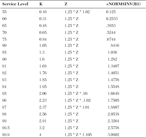
Table 21-1. The Relationship of k to the Z Transform

The way to solve the increase in transportation is to group the forecast by vendor. Tally the vendors’ total overall service level of expected or forecasted out-of-stocks against the vendor predetermined specified service-level objective. After it is determined that total vendor out-of-stocks will fall below the predetermined minimum service level, the vendor will order in quantity. The new formula is Q = d * (LT) + k_v * (LT)^.7. The k_v Service factor is for the vendor and indicates a weighted average of all the k values in the vendor line. It weights the k value by demand and gives an overall service factor for the vendor on all items.

The service-level factor is figured by the sum of the item service-level factors multiplied by demand and divides this by total vendor demand. This gives a prorated vendor service level created by the relative importance of its items. The formula for this is:

If the system forecast of the sum of out-of-stocks for the vendor shows a value lower than the k_v value, it’s time to order. This minimizes the number of shipments because orders are placed only when needed. It is also based on quantifiable measures of vendor service level. To compute the order quantity for each item in the line, match each order quantity against the vendor minimum or EOQ. The process is as follows:

• Average inventory (AI) is computed as 1/2 * OQ.

• The size of each item order is rounded out by the EOQ formula as directed by the next example, where Q_EOQ = |Q/EOQ + .5| * EOQ. The vertical bars indicate an integer value of OQ value rounded by .5.

• The Q_EOQ is the item rounded for the new EOQ.

• Now the average inventory = 1/2 * Q_EOQ.

The EOQ formula is based on a simple formula used to determine the most economical quantity to order so that the total of inventory and setup costs is minimized. The following assumptions are in place:

• Constant per-unit holding and ordering costs

• Constant withdrawals from inventory

• No discounts for large quantity orders

• Constant lead time for receipt of orders

The EOQ is determined as the lowest point on the total cost from Figure 21-1.

There is a relationship between total inventories to the service-level criteria. As the need for higher service level increases, the safety stock begins to increase exponentially. It really takes a turn when it goes above 95% service levels. The values from Table 21-1 give the relationship of k to the Z transform. The k value is plotted against the service level.

Here the EOQ formula transforms from the old version to the new version, which includes the supply chain. The calculations are as follows for the older version:

•

•

•

• The lowest total cost is where the slope is equal to zero. This requires the first derivative of the total cost curve or

• After the differentiation the equation becomes –DS / Q² + H / 2 = 0.

• Now to solve for Q, the formula becomes Q² = 2DS / H.

• The EOQ is the Q calculated as .

For example:

• Suppose annual requirement (AR) = 10,000 units.

• Cost per order (CO) = $2.

• Cost per unit (CU) = $8.

• Carrying cost percentage (percentage of CU) = 0.02.

• Carrying or holding cost per unit = $0.16.

• The freight cost as an average per item = 4%.

• The EOQ = .

• Economic order quantity = 500 units.

Now consider the increase in EOQ and the increased cost of holding the inventory versus the decreased cost of transportation:

• The holding cost is a yearly cost of 16%.

• Freight cost is 4%.

• In this case, do not include the freight in the EOQ calculation. The number of times ordered per year is calculated this way:

N = number of orders per year = D / EOQ = 10,000 / 500 = 20.

As the transportation price increases, the number of inbound shipments will decrease, which begins to make sense using the new EOQ formula.

After the differentiation, this is the formula: −DS / Q² + H / 2 − DFP / Q² = 0. Now it’s time to solve for Q to get the new EOQ formula which takes into account the logistics, or, more specifically, the cost of freight:

There is a shortcut method that can be applied to the old style of calculated EOQ. If the system calculates this EOQ, simply multiply it by a constant coefficient of:

The new EOQ, known as EOQ₁, is calculated as:

where EOQ represents the old style of calculating the economic order quantity.

The following analysis also suggests that as the freight costs increase relative to the cost per order, the importance of transportation becomes more apparent. For instance, if F (freight cost) was 15% instead of 4%, the new EOQ would be 632.

Note that at period 19 on Figure 21-2, the minimum cost for the old EOQ is 77.46154.

Figure 21-2. Plot of the holding and set up cost for the EOQ formula

Figure 21-2 shows the lowest point on the Total Cost Curve to be around period 19.

Figure 21-3, which is an Excel spreadsheet, shows the minimum total cost at period 19 with an EOQ of around 520, which matches the calculation of 516.39. It is the lowest point on the spreadsheet. Close to period 19 the cost gets lower, and after that point the cost begins to rise. The Q on the spreadsheet represents the EOQ.

Figure 21-3. The Excel spreadsheet showing the minimum cost for the EOQ formula

Now consider the new EOQ calculation of including the transportation cost. Assume the following values:

D = 10,000 and S = $2.00 and H = $0.15 and F = .16 and P = 8

Figure 21-4 indicates that the EOQ has shifted from period 19 to around period 33. The top line shows a Minitab line graph showing the minimum at approximately period 33.

Figure 21-4. Shift on minimum to period 33

The Excel spreadsheet in Figure 21-5 shows the new Total Cost at period 33 with the EOQ₁ at around 660, which matches the results on the Excel spreadsheet of 661.31. The Q on the spreadsheet represents the EOQ₁.

Figure 21-5. An Excel spreadsheet showing the minimum at 33

• A 20% decrease in deliveries to and from the supplier to the customer.

• A 20% decrease in the amount of mileage needed to deliver the product from supplier to customer.

• A 20% decrease in the amount of gasoline used from the supplier to the customer.

• A 20% decrease in the amount of CO₂ put into the atmosphere from the decreased usage of gasoline because of the decreased number of deliveries.

Figure 21-6 shows how the freight rate and the number of deliveries are correlated to the freight rate “F.” The chart indicates the number of deliveries that should be made to minimize the total cost of the supply chain. It begins with a freight rate of 1% and then increases by adding 3% to each successive value until it gets to 85%. The freight rate is the Y axis. The graph is calibrated in percentages divided by 10 to make the graph more proportional. A bottom line is F and the top line is N. The F line of 5 is interpreted as a freight rate of 50%. The X axis indicates the number of deliveries per year. Deliveries can be scheduled according to the rate of freight rate increases. For instance, if the freight rate increases from 3.4% to 6.4%, the number of deliveries per year should fall from 16 to 14. This represents an 85% increase in the freight rate, which will cause a 12.5% decrease in the number of deliveries made per year. The data is shown in Table 21-2.

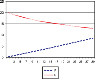
Figure 21-6. The effect of freight rate “F” on number of deliveries “N”

Table 21-2. The Excel Spreadsheet Showing the Effect of Freight Rate “F” on the Number of Deliveries “N”