4
Light measurements
4.1 Units, terminology and calculations
To measure and record light a unit was required that could be understood and repeated experimentally. This was the candle – but not any old candle. It had to be well defined so that it was repeatable (well, almost repeatable). It is quite laughable today to think of a world wide standard measurement of light being dependent on the repeatability of a burning candle, but it is a fact and the specification for the standard candle defined the type of wick and the tallow mixture to be used and the dimensions were an ![]() inch wick and a candle with a diameter of 1
inch wick and a candle with a diameter of 1![]() inches.
inches.
Owing to the unreliability of a wax candle, it was replaced by a lamp burning vaporised pentane with an intensity equal to about 10 of the original candles. Eventually, even this was considered inaccurate and in 1909 a filament lamp was adopted as the standard, which continued until 1948. To enable very accurate measurements to be made, it was decided, at this time, to create a standard based upon the light emitted from a platinum radiator at 1773°C contained within a special vessel. The unit of luminous intensity, the candela, is defined as ‘the luminous intensity, in the perpendicular direction, of a surface of 1/600000 square metres of a blackbody, at the temperature of freezing platinum, under standard atmospheric pressure’.
The radiant flux is the amount of light energy that is given off by an object each second and is measured in ‘joules per second’ (the physical unit of measurement is known as a watt). A 100W lamp therefore, radiates a total of 100 J of light energy each second. However, a 100 W tungsten lamp only radiates approximately 6 W of visible light, the remainder being radiated as non-visible infrared. The more we compress the energy from the light source into the visible spectrum, so we raise the amount of useful watts of light output. Low pressure sodium lamps emit practically all their light at around 590 nm, as this is very close to the peak sensitivity of the eye, it is highly efficient in terms of the number of lumens per watt. Thus, by concentrating the energy into narrow bands, it may be possible to produce light sources with outputs as high as 160 lumens/W and, in fact, it is this type of light generation that is employed in modern high energy light sources such as the HMI, MSR lamps.
As the eye varies in sensitivity with the wavelength of light, it is impractical to use the watt as a measure of the light output, we therefore use the following photometric units which take into account the response of the eye.
Luminous flux measures the total light output of a source and its unit of measurement is the lumen. However, in film and TV we are interested in luminaires that focus the light in a specific direction and light emitted in a specific direction is measured in candelas, and is called the luminous intensity.
Source |
Luminance (in cd/m2) |
Sun |
1600 × 106 |
Crater of Carbon arc |
200 × 106 |
Tungsten lamp (100W clear) |
6.5 × 10⁶ |
Tungsten lamp (100W pearl) |
8 × 10⁴ |
High pressure Mercury lamp (400 W clear) |
120 × 104 |
Fluorescent lamp (80W) |
0.9 × 10⁴ |
Low pressure Sodium lamp (140W clear) |
8 × 10⁴ |
Clear blue sky |
0.4 × 10⁴ |
White paper (reflection factor 80%) illumination 400 lux |
100 |
Grey paper (reflection factor 40%) illumination 400 lux |
50 |
Black paper (reflection factor 4%) illumination 400 lux |
5 |
The incident light striking a unit area is called the illuminance and is measured in lumensm2 (lux). As well as incident light, we are very much concerned with reflected light. The light emitted from a unit area in a specific direction is called luminance and is measured in candelasm2, which indicates how bright an object actually appears, and this may be an illuminated area or the area of a source of light. The luminance of a surface determines how bright that surface actually appears.
1 nit = 1 cdm2
1 footlambert = 3.426 cdm2
1 apostilb = 0.3183 cdm2
Table 4.1 gives the values of luminance for typical sources.
As an example of how we may apply the photometric units in practice, let us consider the light being emitted with a luminous intensity of one candela. The light is assumed to be distributed evenly in all directions, and the two areas shown are representing parts of the inner wall of two spheres, one at one foot from the source and the other at one metre from the source.

Figure 4.1 Candela/lux/foot candle relationship
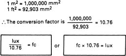
Figure 4.2 Relationship of lux to foot candles
By definition, one foot candle is the amount of light falling on an area of one square foot at a distance of one foot from a source of one candela. The principle is the same for one lux being defined as the amount of light falling on an area of one square metre at a distance of one metre from a source of one candela.
To find the relationship between foot candles and lux, it is necessary to relate the areas being illuminated (see Figure 4.1). By converting the area of one square foot to square millimetres, we have 92 903 mm2 and of course, one square metre is 1 000 000 mm2. If we now divide the larger area by the smaller area we get a factor of 10.76 which is the conversion factor to use when relating foot candles to lux in Figure 4.2.
4.2 Laws – inverse square and cosine
Although there are many ways of reducing the light output of a luminaire, there is not one way of increasing it, therefore our only interest is the reduction of light and the laws that it obeys.

Figure 4.3 Light output
If a diffusion filter or wire gauze is placed in front of a light source, one would expect it to reduce the light output and it is equally obvious that if the material restricts half of the light, then the level will fall by 50% (Figure 4.3). It would appear by similar rationale, that the light from a luminaire would fall off with distance and a common misunderstanding is that at double the distance one would expect to get half the light. This is not so. The light is governed by a simple formula called the ‘Inverse square law’ which states that the light is falling off as the distance squared. Therefore if the distance from the light is doubled, the light will fall to one quarter. It must be said at this point that normal point light sources conform to the inverse square law when calculating illuminance. However, if we look at a larger source area, such as a fluorescent fitting, this needs to be dealt with in a different way. In situations such as this, the inverse square law can be used only if the distance of the light source from the subject is five times the maximum dimension of the source itself. For example, if the source is half a metre across, the inverse square law will only be accurate from a minimum distance of 2.5 m upwards.
![]()
If a light reading is taken at a given distance, say 10 m and has a value of 1000 lux, we can determine the light intensity from the luminaire by simply multiplying the lux reading by the distance squared, i.e. 1000 lux × 102 = 1 00 000 candelas. We now have a constant value for the intensity of the luminaire and it is expressed in candelas. As we arrived at the candela value by multiplying a lux reading by the distance squared, it is equally true that we can divide the candela value by any distance squared and obtain the lux reading at the new distance.
When the incident light falling on a cosine corrected light cell is normal (at 90°) to the plane of the cell, the cell will correctly measure the incident light. If however, the light reaches the cell at any angle other than normal, the amount of light to be measured will change. This variation in light is in direct relation to the angle the light enters the cell, and the light diminishes as the cosine of the angle to the normal and this is known as ‘Lamberts cosine law’. Thus, in theory, light that enters the cell from the side, in other words 90° to the normal would be ‘zero’ on a cosine corrected meter. This variation comes about by the fact that the light has to cover a greater area when striking from any angle other than normal (see Figure 4.4).
Clearly (b) is longer, therefore the hatched area is larger,
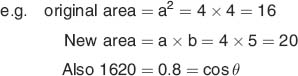
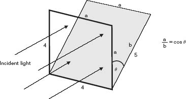
Figure 4.4 Cosine variation
The best example of the spread of light is to consider the follow spot used in a theatre. When normal to a surface it produces a round beam of light. When pointed at an angle to the stage, to cover the artist, the beam is now spread in an elongated shape. The amount of light in the beam has not changed, but the area covered has increased; thus the illumination per unit area has diminished. Obviously, if the beam is elongated more and more as the light approaches from the side, the area covered by the light beam becomes infinite. Thus the amount of light per unit area becomes less and less and approaches zero (Figure 4.5).

Figure 4.5 Incident light level
With very shallow angles to normal, the variations are not significant, but as the angles become greater and approach anything from 45° to 90° quite large variations in light level can occur. This is particularly so when considering outside broadcast lighting and the floodlighting industry have had problems with this phenomenon for many years. Just to give an example, the cosine of 30° = 0.866, the cosine of 45° = 0.77, the cosine of 60° = 0.5, the cosine of 75° = 0.259, the cosine of 90° = zero.
As well as changing in one plane, the light can change in two planes at the same time. The light in the horizontal plane can come in at an angle as well as from the vertical plane, so both our x and y co-ordinates can vary. If this is the case, we have variations of the cosine law from two directions and this is normally called the ‘cosine cubed law’.
4.3 Polar diagrams and their interpretation
We can determine two main important facts about the light output of a luminaire from its polar plot – the intensity of the light and its coverage. All lighting manufacturers use the same system to produce their catalogue information, so it is worth investigating the method of the test to help to understand the results. Whilst light meters are used to read the light arriving at the subject and so provide us with the actual information to work with, it is quite impossible to assess a luminaire against the manufacturer's catalogue information in the same way, because of the variables that must be catered for before a light output comparison can be made.
The supply voltage must be stabilised at the design voltage of the lamp, a 5% reduction at 230 V will result in an approximate light loss of 15%. The lamp used for the test will have been calibrated by the manufacturer, who also supply a laboratory report, showing the exact voltage to run the lamp at to achieve the stated wattage and colour temperature. This sample lamp is kept by the luminaire manufacturer as his standard for all tests (see Figure 4.6).
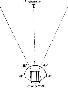
Figure 4.6 Method of producing a polar diagram
When assessing a polar diagram, determine if the manufacturers’ light readings were taken with a wire guard in place; because a 25-mm wire guard will reduce the total light by about 8% – a ploy often used to enhance a products’ specification. When making a polar curve, the luminaire must be checked to see that the reflector is centralised and that the lamp filament is in line with the centre of the reflector. Assuming that lenses and reflectors are clean, then a meaningful test can be made. With the light cell set at the same height as the centre of the luminaire, two methods of test are available to us; a polar test or a flat wall test.
A flat wall test is made by moving a light meter with a cosine corrected cell across a screen at a set distance from the light and readings recorded at regular intervals, keeping the cell parallel to the surface. The most used method is a polar test, where the light is rotated and the cell remains stationary. Then, if flat wall information is required, it can be produced mathematically by applying the Cosine and the inverse square laws. Any tests must be conducted in a darkened room and care must be taken to see that no reflected light from walls or ceiling reach the light cell. The readings can be taken at any distance, however, a very short distance will require very accurate measurements to be made, because any error in the distance will be magnified by the effect of the inverse square law, so that a slight change in distance can produce a large change in the light level.
Typically, luminaires up to 1 kW are measured at 5 m, 1 kW-5kW at 8 m and 10 kW at 10 m, but this is only a guide because the test can be made at any chosen distance. The polar plotter is made up of a stand or platform that will allow the luminaire to rotate. A semicircular scale is placed under the luminaire, equally divided in degrees, and this scale is locked off to the luminaire, so that it rotates with it. A pointer is fixed to the bottom of the support structure so that it remains static. The test can now be made by aligning the centre of the scale with the pointer, and positioning the centre of the light output beam onto the cell. This setting up procedure is usually easier to achieve by first setting the focus to the spot position. The luminaire can now be rotated and readings taken at regular intervals. A typical method is to take readings at every degree for the spot position, and every 2.5° for the full flood position. The centre reading starts at zero degrees and the readings are taken left and right of centre. Having taken the readings and plotted them on a graph, similar to the one illustrated by the Fresnel polar diagram (see Figure 4.8), it is normal to place a mark at the point on the curve that corresponds to 50% of the centre brightness and another mark at 10%. These are known as the ‘beam angle’ and the ‘field angle’ respectively (see Figure 4.7).
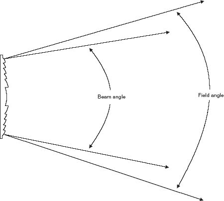
Figure 4.7 Beam and field angles
The significance of the 50% beam angle is that if two lights are required to overlap and provide an even reading across the two distributions they must overlap at the 50% mark to produce 100% to match the centre reading. The 10% mark is normally considered to be the total angle of the light, in view of the fact that any light outside of this reading is of little use.
The readings are taken in lux at a given distance, but are normally quoted in candelas. This is arrived at by multiplying the lux reading by the distance squared from the light to the cell. It is more useful to display the information in candelas because the light level in lux at any distance can be easily calculated by dividing the candela reading by the required distance squared. In this way the manufacturer makes up the typical light output readings in lux at various distances that are used in the catalogue data sheets. Then with a little trigonometry, the diameter can be predicted, given the output angle of the light and the distance. The shape of the flood position in the Fresnel distribution illustrated will produce an even reading across a line 90° to the source. Because the readings are higher either side of the centre this will compensate for the greater distance that the light is projected to reach that part of the distribution.
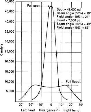
Figure 4.8 Fresnel polar distribution
4.4 The measurement of colour temperature
William Thomson (later to become Lord Kelvin) was an eminent physicist of his day (1824–1907), and was responsible for establishing the Kelvin scale used for colour temperature measurement. Kelvin was faced, when experimenting, with two scales on which temperature could be measured – the Fahrenheit system and the Celsius or, as it is more commonly called – the Centigrade system.
The Fahrenheit system was developed by Daniel Gabriel Fahrenheit (1686–1736), a German physicist who worked in The Netherlands and also invented the alcohol and mercury thermometers. The Fahrenheit scale is based on 32° which represents the freezing point of water and 212° which is the boiling point of water, the interval between these two points being divided into 180 parts or degrees.
The Centigrade system was developed by Anders Celsius (1701–1744), a Swedish professor of astronomy who proposed a temperature scale of 0 to 100 degrees be adopted with 0° as the boiling point of water and 100° as the freezing point.
It was not until after the death of Celsius that Carolus Linnaeus (1707–1778), a Professor of Medicine in Sweden reversed the scale to make the 0° the freezing point and 100° the boiling point. The conversion between the two systems being F = 95 × C° + 32.
Both of these systems were in use for standard temperature readings and both suffered the same problem, namely that the scale did not start at the lowest point of a temperature range and produced negative values.
In their time the scales might have seemed adequate and to represent the Centigrade scale starting at zero, this being the freezing point of water, seemed a good idea. Unfortunately, water freezes at different temperatures at different altitudes and various degrees of purity and quite frankly, has no relevance at all, it could just as easily have been any other substance.
Kelvin decided that both temperature scales were unsuitable for scientific measurements. He had no argument with the Centigrade scale, it was its starting point that caused the problem. Being not only a prominent physicist but a brilliant mathematician, he calculated the theoretical point of absolute zero as being −273° on the Centigrade scale. At this point no material can be further lowered in temperature. This then was his starting point – to set zero on the Kelvin scale at −273° Centigrade, thus from zero upwards getting only positive values.
Since the Kelvin scale is a Centigrade scale displaced from its zero by 273°, a tungsten filament which is glowing and radiating a colour that is 3000 K is burning at a temperature of 2727 °C.
The Kelvin colour temperature scale can only be used when measuring a source that emits energy in a continuous spectrum and approximates to a blackbody radiator such as a tungsten filament, or the ultimate in light sources, the sun.
What this means is that a lamp with a 2700 K colour temperature produces approximately the same spectrum of light as a blackbody at 2700 K. (Most hot objects do not follow Planck's blackbody radiation law: only perfectly black objects do). If we examine the visible spectrum portion of the blackbody curves given it will be seen that the curves are continuous over the visible wavelengths. As the object becomes hotter, it is noticeable that the amounts of red energy and blue energy are varying in relation to each other. If we could have a meter which measured the ratio of the red/blue balance, we would then have a reasonably close approximation to blackbody temperatures. In fact, the older style of colour temperature meters made throughout the world generally worked on the fact that they employed a red and blue filter to measure the relative amounts of each and thus find the corresponding colour temperature.
The colour of light emitted from a discharge lamp cannot be expressed in Kelvins because the spectral output in the lamp is not continuous but dependent on the gases and rare earths used in its manufacture to introduce the required additional colours which help to create the colour of the source (see Figure 4.9), and the compounds used emit colours in only comparatively narrow bands. In photographic and TV cameras the film stock and the colour receptors are responsive to the amounts of red, green and blue in the light, but unfortunately due to the spiky nature of the colour distribution from a discharge lamp a standard colour meter that measures only the red/blue balance of a source will give erroneous readings because it is not measuring the total spectral output.
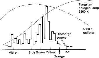
Figure 4.9 Comparison of discharge and incandescent sources
4.5 Types of meter
Luminance (reflected) light meters
Photographic meters, either the built in type as with most modern 35-mm cameras, or a hand held meter, measure the reflected light from the scene which is going to reach the film. As the film has a certain sensitivity, either the stop and/or the speed of the shutter have to be adjusted so that the correct quantity of light reaches the emulsion, so that well exposed pictures are produced. Of course, nowadays, most cameras do everything automatically. The basis of reflected light measurements is an 18% reflectance value which produces an average brightness standard of measurements for film and TV cameras. At this point it must be stated that we are only measuring the amount of light, not the colour of the source, as long as the meter responds faithfully to all visible wavelengths. If we have a red card that reflects 18% of the light striking it or we have a green card with the same reflectance, they will appear to be the equivalent as far as a camera is concerned because we haven't taken any account of the colour involved. We have all been caught out by taking pictures of snow scenes or pictures in very dark areas when the average brightness cannot equate the scenic values very accurately to the 18% reflectance.
Luminance meters are used for the measurement of a light source or surface brightness. Two of the most important factors with a luminance meter is the angle of acceptance so it can cover very small areas at a distance and secondly, is to ensure that there is no light entering the cell outside the angle of acceptance, which would give false readings. For average use, an acceptance angle of one degree is acceptable, however for very accurate luminous measurements on small areas one third of a degree is possible in some meters. A normal luminance meter will be calibrated in candelas per metre squared and alternatively foot lamberts. Photographic luminance meters will have systems where film speed and other parameters can be entered so that an exposure value can be obtained from the meter readings. In addition to a standard luminance meter, it is now possible to obtain meters where the measurements of the colour tri-stimulus values are made in addition to the candela per metre squared units or foot lamberts. These meters would be used where the light sources are too small to be measured with standard colorimeters, for example, LEDs and small lamps. They are also useful to measure light sources when they are operating and obviously very hot. Further use is for inaccessible or distant light sources, and some meters allow accurate measurements of areas as small as 1.3 mm in diameter.
Illuminance (incident) light meters
A better way of measuring the amount of light is by taking incident light readings which are not influenced by the subject matter itself. If we measure incident light, it is then up to the operator to adjust the equipment being used to give a balanced exposure on the scene itself. A good modern incident light meter should be capable of measuring the luminance in either lux or foot candles. In addition, it's much better if the meter has a digital readout so the figures are accurately displayed. The spectral response must match within fairly close limits the CIE photopic luminosity curve which gives the correct assessment of colour balance for incident light readings (see Figure 4.10).
In our measurement of incident light, it is essential that we use a cosine corrected cell which gives readings which are correct and take into account the angle of the light incident on the meter. It is also important that the meter would be facing the direction of the most interest visually, i.e. along the path that the camera would look at the scene. When taking measurements on vertical or horizontal surfaces, the meter should be parallel to the surface.
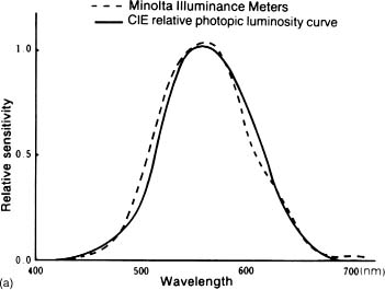
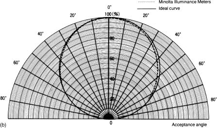
Figure 4.10 (a) Incident light meter – spectral response; (b) Incident light meter – acceptance angle characteristics (courtesy of Minolta (UK) Ltd)
Tri-stimulus colour meter
In film and TV we need accurate measurements of incident light onto subjects. We also need an accurate measure of colour temperature if we are using sources that approximate to the blackbody curve and there is also a need to measure colour accurately so that errors are avoided when operating discharge sources in either film or TV. A tri-stimulus meter is really a clever little hand held computer. It contains three photo cells which are filtered to detect the primary stimulus values of blue, green and red light under a special opal diffuser. This diffuser is specially made to take account of the direction of light and therefore inherently calculates the cosine angle of incident light. The incident light level can be derived from the output of the green photo cell as this relates to the photopic curve. It would appear that only the blue and red photo cells would be required to give a colour temperature reading; however meters of this type will compute a point on the spectrum locus from an analysis of the red, blue and green receptors. A big advantage of using meters such as this, is that colour shifts can be accurately measured by using the x and y co-ordinates on a CIE spectral diagram. Readings can be assigned a ‘K’ output reading signifying colour temperature, but it may be that the meter is measuring a discharge source. This can be given a correlated colour temperature. The correlated colour temperature is the nearest point on the blackbody locus which matches the source. The measurements always have to be referred back to the x y co-ordinates to get an accurate representation from the CIE diagram. Meters such as this although relatively expensive compared with a basic incident light meter, are invaluable and in fact, indispensable to the assessment of any lighting.