CHAPTER 2

FIRST-ORDER LOGIC

2.1 LANGUAGES

We developed propositional logic to model basic proof and truth. We did so by using propositional forms to represent sentences that were either true or false. We saw that propositional logic is consistent, sound, and complete. However, the sentences of mathematics involve ideas that cannot be fully represented in propositional logic. These sentences are able to characterize objects, such as numbers or geometric figures, by describing properties of the objects, such as being even or being a rectangle, and the relationships between them, such as equality or congruence. Since propositional logic is not well suited to handle these ideas, we extend propositional logic to a richer system.

Predicates

Consider the sentence it is a real number. This sentence has no truth value because the meaning of the word it is undetermined. As noted on page 3, the word it is like a gap in the sentence. It is as if the sentence was written as

However, that gap can be filled. Let us make some substitutions for it:

5 is a real number.
π/7 is a real number.
Fido is a real number.
My niece's toy is a real number.

With each replacement, the word that is undetermined is given meaning, and then the sentence has a truth value. In the examples, the first two propositions are true, and the last two are false.

Notice that changes, whereas is a real number remains fixed. This is because these two parts of the sentence have different purposes. The first is a reference to an object, and the second is a property of the object. What we did in the examples was to choose a property and then test whether various objects have that property:

Depending on the result, these two parts are put together to form a sentence that either accurately or inaccurately affirms that a particular property is an attribute of an object. For example, the first sentence states that being a real number is a characteristic of 5, which is correct, and the last sentence states that being a real number is a characteristic of my niece's toy, which is not correct. We have terminology for all of this.

• The subject of a sentence is the expression that refers to an object.
• The predicate of a sentence is the expression that ascribes a property to the object identified by the subject.

Thus, 5, π/7, Fido, and my niece's toy are subjects that are substituted for it, and is a real number is a predicate.

Substituting for the subject but not substituting for the predicate is a restriction that we make. We limit the extension of propositional logic this way because it is to be part of mathematical logic and this is what we do in mathematics. For example, take the sentence,

On its own it has no truth value, but when we substitute x = 5 or x = 10, the sentence becomes a proposition. In this sense, x + 2 = 7 is like it is a real number. Both the sentences have a gap that is assigned a meaning giving the sentence a truth value. However, the mathematical sentence is different from the English sentence in that it is unclear as to what part is the subject. Is it x or x + 2? For our purposes, the answer is irrelevant. This is because in mathematical logic, the subject is replaced with a variable or, sometimes, with multiple variables. This change leads to a modification of what a predicate is.

DEFINITION 2.1.1

A predicate is an expression that ascribes a property to the objects identified by the variables of the sentence.

Therefore, the sentence x + 2 = 7 is a predicate. It describes a characteristic of x. When expressions are substituted for x, the resulting sentence will be either a proposition that affirms that the value added to 2 equals 5 or another predicate. If x = 5 is substituted, the result is the true proposition 5 + 2 = 7. That is, x + 2 = 7 is satisfied by 5. If x = 10 and the substitution is made, the resulting proposition 10+2 = 7 is false. In mathematics, it is also common to substitute with undetermined values. For example, if the substitution is x = y, the result is the predicate y + 2 = 7, and if the substitution is x = sin θ, the result is the predicate sin θ + 2 = 7. Substituting x = y + 2z² yields y + 2z² + 2 = 7, a predicate with multiple variables. If we substitute x = y² − 7y, the result is y² − 7y + 2 = 7, which is a predicate with multiple occurrences of the same variable.

Assume that x represents a real number and consider the sentence

Although there is a variable with 2 occurrences, the sentence is a proposition, so in propositional logic, it is an atom and would be represented by P. This does not tell us much about the sentence, so we instead break the sentence into two parts:

A quantifier indicates how many objects satisfy the sentence. In this case, the quantifier is the existential quantifier, making the sentence an existential proposition. Such a proposition claims that there is at least one object that satisfies the predicate. In particular, although other sentences mean the same as (2.1) assuming that x represents a real number, such as

and

they all claim along with (2.1) that there is a real number x such that x + 2 = 7. This is true because 5 satisfies x + 2 = 7 (Figure 2.1).

Figure 2.1

Again, assume that x is a real number. The sentence

claims that x + 5 = 5 + x is true for every real number x. To see this, break (2.2) like (2.1):

This quantifier is called the universal quantifier. It states that the predicate is satisfied by each and every object. Including propositions that have the same meaning as (2.2), such as

and

(2.2) is true because each substitution of a real number for x satisfies the predicate (Figure 2.2). These are examples of universal propositions,.

A proposition can have multiple quantifiers. Take the equation y = 2x² + 1. Before we learned the various techniques that make graphing this equation simple, we graphed it by writing a table with one column holding the x values and another holding the y values. We then chose numbers to substitute for x and calculated the corresponding y. Although we did not explicitly write it this way, we learned that

This is a universal proposition, and its predicate is

Figure 2.2

We conclude that (2.3) is true because whenever x is replaced with any real number, there is a real number y that satisfies y = 2x² + 1.

The symbolic logic that we define in this chapter is intended to model propositions that have a predicate and possibly a quantifier. As with propositional logic, an alphabet and a grammar will be chosen that enable us to write down the appropriate symbols to represent these sentences. Unlike propositional logic where we worked on both its syntax and semantics at the same time, this logic starts with a study only of its syntax.

Alphabets

No matter what mathematical subject we study, whether it is algebra, number theory, or something else, we can write our conclusions as propositions. These sentences usually involve mathematical symbols particular to the subject being studied. For example, both (2.1) and (2.2) are algebraic propositions. We know this because we recognize the symbols from algebra class. For this reason, the symbolic logic that we define will consist of two types of symbols.

DEFINITION 2.1.2

Logic symbols consist of the following:

Theory symbols consist of the following:

It is not necessary to choose any theory symbols. However, if there are any, theory symbols must be chosen so that they are not connectives, quantifier symbols, the equality symbol, or grouping symbols, and the selection of theory symbols has precedence over the selection of variable symbols. This means that these two collections must have no common symbols. Moreover, although this is not the case in general, we assume that the logic symbols that are not variable symbols will be the same for all applications. On the other hand, theory symbols (if there are any) vary depending on the current subject of study. A collection of all logic symbols and any theory symbols is called a first-order alphabet and is denoted by A.

The term theory refers to a collection of propositions all surrounding a particular subject. Since different theories have different notation (think about how algebraic notation differs from geometric notation), alphabets change depending on the subject matter. Let us then consider the alphabets for a number of theories that will be introduced later in the text. The foundational theory is the first example.

EXAMPLE 2.1.3

Set theory is the study of collections of objects. The ∈ is the only relation symbol, and it is binary. It has no other theory symbols. The theory symbols of set theory are denoted by ST and are summarized in the following table.

EXAMPLE 2.1.4

Number theory is the study of the natural numbers. The symbols + and · represent regular addition and multiplication, respectively. As such they are binary function symbols. These and its other theory symbols are indicated in the following table and are denoted by NT.

Another approach to number theory is called Peano arithmetic (Peano 1889). It is the study of the natural numbers using Peano's axioms. It has a constant symbol 0 and a unary function symbol S. Denote these symbols by AR.

The Peano arithmetic symbols are sometimes extended to include symbols for the operations of addition and multiplication and the less-than relation. Denote this extended collection by AR′.

EXAMPLE 2.1.5

Group theory is the study of groups. A group is a set with an operation that satisfies certain properties. Typically, the operation is denoted by the binary function symbol . There is also a constant represented by e. Ring theory is the study of rings. A ring is a set with two operations that satisfy certain properties. The operations are usually denoted by the binary function symbols ⊕ and ⊗. The constant symbol is . These collections of theory symbols are denoted by GR and RI, respectively, and are summarized in the following tables.

Field theory is the study of fields. A field is a type of ring with extra properties, so the theory symbols RI can be used to write about fields. However, if an order is defined on a field, a binary relation symbol is needed, and the result is the theory of ordered fields. Denote these symbols by OF.

Notice that the collections of theory symbols in the previous examples had at most two constant symbols. This is typical since subjects of study usually have only a few objects that require special recognition. However, there will be times when some extra constants are needed to reference objects that may or may not be named by the constant theory symbols. To handle these situations, we expand the given theory symbols by adding new constant symbols.

DEFINITION 2.1.6

Let A be a first-order alphabet with theory symbols S. When constant symbols not in S are combined with the symbols of S, the resulting collection of theory symbols is denoted by . The number of new constant symbols varies depending on need.

For example, suppose that we are working in a situation where we need four constant symbols in addition to the ones in OF. Denote these new symbols by c₁, c₂, c₃, and c₄. Then, consists of these four constant symbols and the symbols from OF.

Terms

For a string to represent a proposition or a predicate from a particular theory, each nonlogic symbol of the string must be a theory symbol of that subject. For example,

and

are strings for set theory. However, some strings have a reasonable chance of being given meaning, others do not. As with propositional logic, we need a grammar that will determine which strings are legal for the logic. Because a predicate might have variables, the types of representations that we want to make are more complicated than those of propositional logic. Hence, the grammar also will be more complicated. We begin with the next inductive definition (compare page 59).

DEFINITION 2.1.7

Let A be a first-order alphabet with theory symbols S. An S-term is a string over A such that

Denote the collection of strings over A that are S-terms by TERMS(A).

The string ft₀t₁ · · · t_n−1 is often written as f(t₀, t₁,..., t_n−1) because it is common to write functions using this notation. We must remember, however, that this notation can always be replaced with the notation of Definition 2.1.7. Furthermore, when writing about a general S-term where it is not important to mention S, we often simply write using the word term without the S. We will follow this convention when writing about similar definitions that require the theory symbols S.

EXAMPLE 2.1.8

Here are examples of terms for each of the indicated theories. Assume that x, y and z₁ are variable symbols.

The string +xy is typically written as x + y, and the string 0a₁ is typically written as 0 a₁. If NT is expanded to by adding the constants c and d, then +cd is an -term.

As suggested by Example 2.1.8, the purpose of a term is to represent an object of study. A variable symbol represents an undetermined object. A constant symbol represents an object that does not change, such as a number. A function symbol is used to represent a particular object given another object. For example, the NT-term +x2 represents the number that is obtained when x is added to 2.

Formulas

As propositional forms are used to symbolize propositions, the next definition is the grammar used to represent propositional forms and predicates. The definition is given inductively and resembles the parentheses-less prefix notation invented by Łukasiewicz (1951) in the early 1920s.

DEFINITION 2.1.9

Let S be the theory symbols from a first-order alphabet A. An S-formula is a string over A such that

The string Rt₀t₁ · · · t_n−1 is often represented as R(t₀, t₁,..., t_n−1). A formula of the form ∀xp is called a universal formula, and a formula of the form ∃xp is an existential formula. Parentheses can be used around an S-formula for readability, especially when quantifier symbols are involved. For example, ∀x∃yp is the same formula as ∀x(∃yp) and ∀x∃y(p).

EXAMPLE 2.1.10

Let x and y be variable symbols. Let c be a constant symbol; f, g, and h be unary function symbols; and R be a binary relation symbol from S. The following are S-formulas.

In practice, Rc f y is usually written as R(c, f(y)), ¬(y = gc) as y ≠ g(c), Rx f x as R(x, f (x)), Rfxx as R(f(x), x), and Rfxgy as R(f(x), g(y)).

EXAMPLE 2.1.11

These are some ST-formulas with their standard translations.

EXAMPLE 2.1.12

Here are some NT-formulas with their corresponding predicates.

We now name the system just developed.

DEFINITION 2.1.13

An alphabet combined with a grammar is called a language. The language given by Definitions 2.1.2 and 2.1.9 is known as a first-order language. A formula of a first-order language is a first-order formula, and all of the formulas of the first-order language with theory symbols S is denoted by L(S).

The first-order language developed to represent predicates, either with quantifiers or without them, is summarized in Figure 2.3. An alphabet that has both logic and theory symbols is chosen. Using a grammar, terms are defined, and then by extending the grammar, formulas are defined. A natural question to ask regarding this system is what makes it first-order? Look at the last part of Definition 2.1.9. It gives the rule that allows the addition of a quantifier symbol in a formula. Only ∀x or ∃x are permitted, where x is a variable symbol representing an object of study. Thus, only propositions that begin as for all x ... or there exists x such that ... can be represented as a first-order formula. To quantify over function and relation symbols, we need to define a second-order formula. Augment the alphabet A with function and relation symbols, which creates what is know as a second-order alphabet, and then add

and

to Definition 2.1.9. For example, if the first-order formula

is intended to be true for any A and B, it can be written as the second-order formula

where Ax represents the relation x ∈ A and Bx represents the relation x ∈ B.

Figure 2.3 A first-order language.

Exercises

1. Determine whether the given strings are GR-terms. If a string is not a GR-term, find all issues that prevent it from being one.

(a) 2e

(b) xy

(c)

(d) <xe

(e) xye

2. Write the GR-terms from Exercise 1 in their usual form (Example 2.1.10).

3. Extend ST to ST′ by adding the constant symbol ∅ and the unary function symbol P. Determine whether the given strings are ST′-terms. If a string is not a ST′-term, find all issues that prevent it from being one.

(a) ∈x∅

(b) ∅

(c) x

(d) P∈xy

(e) Px

4. Determine whether the given strings are OF-formulas. If a given string is not a OF-formula, find all issues that prevent it from being one.

(a) < ⊕xy⊗xy

(b) ⊕x = ⊗y

(c) ∀x∃y(+xy = 0)

(d) ∀x∀y(⊗xy = ⊕yx) → <xy

(e) ¬(<⊗xy ∧ ⊕xy) ↔ ∀u∀v(<⊗xy⊕uv)

5. Write the RI-formulas from Exercise 4 in their usual form.

6. Extend ST to ST″ by adding the constant symbol ∅ and the binary relation symbol R. Determine whether the given strings are ST″-formulas. If a given string is not a ST″-formula, find all issues that prevent it from being one.

(a) Rx∅ ∨ ∈xy

(b) Rx∅ → ∈+xyz

(c) ∀x∃∅ (¬∈x∅)

(d) ∀x ∨ ∀y ∨ ∀z(∈∅xyz)∨ ∈ ∅∅

(e) [∃x(Rx∅) → ∃u∃v∃w(¬∈uv ↔ ¬∈uw)] ∨ ∅ = x₁

7. Write the ST″-formulas from Exercise 6 in their usual form.

8. Translate the given sentence to an S-formula for the given theory symbol.

(a) For all x, S(x) ≠ 0. (S = AR)

(b) For every number x, there is a number y such that x y = e. (S = GR)

(c) If x < y and y < z, then x < z. (S = OF)

(d) It is false that x ∈ y, y ∈ z, and z ∈ x for all x, y, and z. (S = ST)

(e) For every u and v, there exists w such that if u = v, then u + w = v + w. (S = RI and + should be translated as ⊕ in the RI-formula.)

9. Extend NT to NT′ by adding the numerals 2, 3,..., 9. Answer the following questions.

(a) Is +34 = 7 a NT′-term? Explain.

(b) Is ·4+39 a NT′-term? Explain.

(c) Is ∃x(+·4x8 = +3x) a NT′-formula? If it is, find x.

(d) If possible, give an example of a NT-formula that is not a NT′-formula.

(e) If possible, give an example of a NT′-formula that is not a NT-formula.

2.2 SUBSTITUTION

As noted in the beginning of Section 2.1, there are times when a substitution will be made for a predicate's variable. For example, in algebra, if f(x) = 3x² + x + 1, then f(y) = 3y² + y + 1, f(2) = 3(2)² + 2 + 1, and f(sin x) = 3 sin² x + sin x + 1. That is, we can substitute with variables, constants, and the results from functions. Therefore, to represent this in formulas, we can replace a variable with a term.

Terms

We begin by defining what it means to substitute for a variable in a term. We use ⇔ because one string can be replaced with the other string.

DEFINITION 2.2.1 [Substitution in Terms]

Let S be theory symbols from a first-order alphabet A. Let x be a variable symbol from A and t be an S-term. The notation

means that x is replaced with t at every appropriate occurrence of x. For terms, this means the following.

Observe that when a substitution of a term is made into a term, the result is another term.

EXAMPLE 2.2.2

Let x, y, and z be distinct variable symbols; c and d be constant symbols; f be a binary function symbol; and g and h be unary function symbols. This means that fcggd is typically written as f(c,g(g(d))).

Free Variables

Substitution for a variable in a formula is a bit more involved. This is because of the influence of any possible quantifiers. For example, take the formula

By Definition 2.2.1, we know that we can substitute constants c for x and d for y in the terms x, y, and fy. We expect that we should also be able to make this substitution into the formula resulting in

However, in the formula

the situation is different because of the quantifiers. Consider the corresponding occurrences in (2.4) and its quantified (2.5):

Even though each occurrence of x and y in (2.4) can receive a substitution, each corresponding occurrence in (2.5) cannot because of the quantifiers.

DEFINITION 2.2.3

Let S be theory symbols. Let t₀, t₁, ... , t_n−1 be S-terms, R be an n-ary relation symbol from S, and p and q be S-formulas. An occurrence of a variable in a formula is free or not free only according to the following rules:

If an occurrence of a variable is not free, it is bound. All free occurrences of x in p are within the scope of the universal quantifier in ∀xp and the existential quantifier in ∃xp.

EXAMPLE 2.2.4

Let f be a unary function symbol and R be a 3-ary relation symbol. In the formula

all occurrences of x and y are bound, but the occurrence of z is free. In the formula

all occurrences of x and z are free, but the occurrences of y are bound. In

all occurrences are free because all occurrences are free in x = y, fx = y, and Rxyz.

We need to know whether a formula has a free occurrence of a variable, so we make the next definition.

DEFINITION 2.2.5

A free variable of the S-formula p is a variable that has a free occurrence in p.

EXAMPLE 2.2.6

Using the f and R from Example 2.2.4, both x and y are free variables of the formula

even though x has both free and bound occurrences.

Formulas

We can now define what it means to make a substitution into a formula.

DEFINITION 2.2.7 [Substitution in Formulas]

Let S be theory symbols from a first-order alphabet A. Let x and y be variable symbols of A and R be an n-ary relation symbol from S. Suppose that p and q are S-formulas and t, t₀, t₁,..., t_n−1 are S-terms.

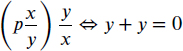
The condition on the term t in the last two parts of Definition 2.2.7 is important. Consider the RI-formula

The usual interpretation of p is that given x, there exists an number y such that x+y = 0. Let f be a unary function symbol and z be a variable symbol. Since y is not a symbol of z,

which has the same standard interpretation as p. Since y is not a symbol of fz, we can substitute to find that

This is a reasonable substitution because it states that for the number given by fz, there is a number y that when added to fz gives 0. This is very similar to the standard interpretation of p. Both of these substitutions work because the number of free occurrences is unchanged by the substitution. However, if we allow the term to include y among its symbols, the substitution would yield

The typical interpretation of (2.6) is that there exists a number y such that y + y = 0. This is a reasonable proposition, but not in the spirit of the original formula p. The change of interpretation is due to the change in the number of free occurrences. The formula p has one free occurrence, while (2.6) has none. Therefore, when making a substitution, the number of free occurrences should not change, and for this reason,

EXAMPLE 2.2.8

Let p be the NT formula

Notice that x₂ is a free variable of p. However, all occurrences of x₀ and x₁ are bound. Therefore,

and then letting y be a variable symbol,

and finally,

This last formula has no free variables. A standard interpretation of this formula is

for every integer x₀ and x₁, if x₀ = x₁, then x₀ + 1 = x₁ + 1.

Furthermore,

Let p represent the NT-formula +y2 = 7. Observe that p has y as a free variable. To emphasize this, instead of writing

we often denote the formula by p(y) and write

Although x is not a variable in the equation, we can also write

For example, if we wanted to interpret the formula as an equation with one variable, we would use p(y). If we wanted to view it as the horizontal line y = 5, we would use q(x, y).

DEFINITION 2.2.9

Let A be a first-order alphabet with theory symbols S. Let p be an S-formula. If p has no free variables or the free variables of p are among the distinct variables x₀, x₁,..., x_n−1 from A, define

The notation of Definition 2.2.9 can also be used to represent substitutions. Consider the formula p := x + y = 0. Observe that

and

However, suppose that we want to substitute into p so that the result is y + x = 0. To accomplish this, we need two new and distinct variable symbols, u and v. Then,

and then,

Therefore,

This works because in (2.7), each variable symbol is replaced by a new symbol in such a way that the resulting formula has the same meaning as the original. In this way, when the original variable symbols are brought back in (2.8), all of the substitutions are made into distinct variables so that there are no conflicts and the switch can be made. This process can be generalized to any number of variable symbols in any order.

DEFINITION 2.2.10

Let p(x₀, x₁,..., x_n−1) be an S-formula and u₀, u₁,..., u_n−1 be distinct variable symbols not among x₀, x₁,..., x_n−1. Define

Then, for all S-terms t₀, t₁,..., t_n−1, define

This is called a simultaneous substitution and is equivalent to replacing all free occurrences of x₀, x₁,..., x_n−1 in p with t₀, t₁, ..., t_n−1, respectively.

Observe that if p does not have free variables, then p(t₀, t₁,..., t_n−1) ⇔ p.

EXAMPLE 2.2.11

To illustrate Definition 2.2.10, let RI′ be the theory symbols of RI combined with constant symbols 1 and 2. Let p be the RI′-formula

Since x, y, and z are free variables, represent p by p(x, y, z, w). Then,

EXAMPLE 2.2.12

Let S have constant symbols 5 and 9. Define p(x, y) to be the S-formula

The first occurrence of y is free, and since ∀x applies only to variables within the brackets on the left, the last occurrence of x is also free. Therefore, p(x, y) is the disjunction of two formulas that we call u(y) and v(x):

from which we derive

As in Example 2.2.11, finding p(9, 5) is equivalent to simply replacing the free occurrences of x with 9 and the occurrences of y with 5.

EXAMPLE 2.2.13

Consider the NT-formula,

which is often written as

The formula within the scope of the first quantifier symbol in (2.10) is

Notice that the occurrences of x are free in (2.11), but the occurrences of y and z are bound. For example, we can make the substitution

Now, letting

we have that p(x) ⇔ ∀yq(x, y). We can also define

so that q(x, y) ⇔ ∀zr(x, y, z). What we have done is to break apart an NT-formula that contains multiple quantifiers into a sequence of formulas:

We conclude that (2.10) can be written as

or

Observe that (2.9) has no free variables. It is a type of formula of particular importance because it represents a proposition. In other words, (2.9) is a propositional form.

DEFINITION 2.2.14

An S-formula with no free variables is called an S-sentence.

Exercises

1. Given a term, make the indicated substitution.

2. Given a formula, make the indicated substitution.

3. Identify all free occurrences of x in the given formulas.

(a) x + 4 < 10

(b) ∃x∀y(x + y = 0)

(c) ∀x∀y(x + y = y + x) ∨ ∀z(x + y = z − 3)

(d) ∀x[∀z∀y(x + y = 2 · z) ↔ x + x = 2 · x]

4. Identify all bound occurrences of x in the given formulas.

(a) (∀x) [p(x) → (∃y)q(y)]

(b) (∃x)p(x, y) → (∀y)q(x)

(c) (∃x)(x > 4) ∧ x < 10

(d) [(∀x)(x + 3 = 1) ∧ x = 9] ∨ (∃y)(x < 0)

5. Make the simultaneous substitution p(a) for each of the given formulas.

(a) p(x) := 2x + a = 9

(b) p(x) := ∀x(x + y = y + x)

(c) p(x) := ∃xq(x) → ∀yr(x, y)

(d) p(x) := x + 4 = 0 ∧ ∃x(y + z = x) ∨ ∃z(x + z = 3)

6. Make the simultaneous substitution q(1,2,3) for each of the given formulas.

(a) q(x, y, z) := u + v + w

(b) q(x, y, z) := r(x, y) → (∀x) [p(x) ∧ (∃y)t(y, z)].

(c) q(x, y, z) := ∃x(x + y = z) ∧ ∀y(x + y + z) ∨ ∀x∀y(x + y + z)

(d) q(x, y, z) := ∃x[p(x) ∧ ∀y(p(x) ∧ p(y) → x = y ∨ y = z)]

7. Identify the formula to the right of each quantifiers in the given formulas.

(a) (∀x) [p(x) → (∃y)q(y)]

(b) (∃x) p(x, y) → (∀y)q(y)

(c) (∀x)(∃y)(∃z)p(x, y, z) ∧ r(w)

(d) p(x) ∧ (∃x)(∀y)q(x, y) ∨ (∀z)r(z)

8. Which of the following are sentences.

(a) ∀x∀y[q(x) ∨ r(y)] ⇒ ∀y[q(a) ∨ r(y)]

(b) q(2) ∧ t(3) ⇒ ∃y[q(2) ∧ t(y)]

(c) ∃w[∃x[p(x) ∨ ∃zq(z) ↔ ∃y[p(x) ∧ q(y)] → ∀xr(x)] → ∀yr(x)]

(d) ∀x∀y(p(x) → [q(y) ∧ r(z)]) → ∃x¬q(x)

2.3 SYNTACTICS

Since formulas without free variables are propositional forms, we can write proofs involving them using the rules from Sections 1.2 through 1.4. However, since the inference rules did not involve quantification, we need new rules to deal with universal and existential formulas. We need rules covering not only negations but also rules that enable the removal (instantiation) and adjoining (generalization) of quantifiers. We add these rules to Definition 1.2.13 to obtain a stronger notion of proof. Furthermore, since every sentence is a propositional form, every reference to a propositional form in Definition 1.2.13 can be considered to be a reference to a sentence. This allows us to write formal proofs using first-order languages.

Quantifier Negation

Consider the proposition

all rectangles are squares.

This sentence is false because there is a rectangle in which one side is twice the length of the adjacent side, so

not all rectangles are squares.

That is,

some rectangle is not a square

is true. Generalizing, we conclude that

the negation of all P are Q is some P are not Q.

This should be translated as an inference rule for formulas, so we assume

Now consider the proposition

some rectangles are round.

This is false because there are no round rectangles, so

all rectangles are not round

is true. Generalizing, we conclude that

the negation of some P are Q is all P are not Q.

Again, this should be translated as an inference rule for formulas, so we assume

Figure 2.4 The modern square of opposition.

Furthermore, by DN and (2.13),

and by DN with (2.12),

We summarize assumptions (2.12) and (2.13) and the two conclusions in the following replacement rule.

REPLACEMENT RULES 2.3.1 [Quantifier Negation (QN)]

Let S be theory symbols and p be an S-formula.

QN is illustrated with the modern square of opposition (Figure 2.4). Negations of quantified formulas are found at opposite corners. A version of the Square is found in Aristotle's De Interpretatione, dating around 350 BC (Aristotle 1984).

Whenever we negate formulas of the form ∀xp or ∃xp, to make it easier to read, the final form should not have a negation immediately to the left of any quantifier, and using the replacement rules, the negation should be as far into the formula p as possible. We say that such negations are in positive form.

EXAMPLE 2.3.2

Find the negation of ∀x(p ∧ q) and put the final answer in positive form.

The next example will use De Morgan's law as the last one did. It also needs material implication and double negation.

EXAMPLE 2.3.3

Find the negation of ∀x∃y[p(x) → q(y)] and put it into positive form.

Proofs with Universal Formulas

Consider the sentence all multiples of 4 are even. This implies, for instance, that 8, 100, and −16 are even. To generalize this reasoning to formulas means that whenever we have ∀xp(x), we also have p(a), where a might be either a constant symbol such as 8, 100, and −16 or a randomly chosen constant symbol. This gives the first inference rule that involves a quantifier. We do not prove it, but take it to be an axiom. Observe the use of Definition 2.1.6

INFERENCE RULE 2.3.4 [Universal Instantiation (UI)]

If p(x) is an S-formula, then for every constant symbol a from ,

We make two observations about UI. First, since the resulting formula is to be part of a proof, the substitution must yield a sentence, so a must be a constant symbol. Second, we use the notation p(x) to represent the formula instead of p because ∀xp(x) will be part of a proof, which means, again, that it must be a sentence. Writing p(x) limits the formula to have only x as a possible free variable, so ∀xp(x) is a sentence. If the formula p had free variables other than x, then ∀xp would not be a sentence and not suitable for a proof.

EXAMPLE 2.3.5

Let p, q, and r be S-formulas and a and b be constant symbols from . The following are legitimate uses of UI. Notice that each of the inferences results in an -formula.

Before we can write formal proofs, we need a rule that will attach a universal quantifier. It will be different from universal instantiation, for it requires a criterion on the constant.

DEFINITION 2.3.6

Let a be a constant symbol introduced into a formal proof by a substitution. If the first occurrence of a is in a sentence that follows by UI, then a is arbitrary. Otherwise, a is particular and can be denoted by â to serve as a reminder that the symbol is not arbitrary.

The idea behind Definition 2.3.6 is that if a constant symbol a is arbitrary, it represents a randomly selected object, but if a is particular, then a represents an object with at least one known property. This property can be identified by a formula p(x) so that we have p(a).

EXAMPLE 2.3.7

The constant symbol a in the following is not arbitrary because its first occurrence of a in line 1 is not the result of UI.

Therefore, these two lines should be written using â instead of a.

However, a in the following is arbitrary because its first occurrence is in line 2, and line 2 follows from line 1 by UI.

We can now introduce the rule of inference that allows us to attach universal quantifiers to formulas. We state it as an axiom.

INFERENCE RULE 2.3.8 [Universal Generalization (UG)]

If p(x) is an S-formula with no particular constant symbols and a is an arbitrary constant symbol from ,

Consider the following argument:

All squares are rectangles.

All rectangles are quadrilaterals.

Therefore, all squares are quadrilaterals.

Representing the premises by ∀x[s(x) → r(x)] and ∀x[r(x) → q(x)], a formal proof of this includes UG:

Since a was introduced in line 3 by UI, it is an arbitrary constant symbol. In addition, s(a) → q(a) contains no particular constant symbols that appeared in the proof by substitution. Hence, the application of UG in line 6 is legal.

EXAMPLE 2.3.9

These are illegal uses of universal generalization.

Now for some formal proofs.

EXAMPLE 2.3.10

Prove: ∀x∀yp(x, y) ∀y∀xp(x, y)

Since both a and b first appear because of UI, they are arbitrary and universal generalization can be applied to both constant symbols.

EXAMPLE 2.3.11

Prove: ∀x [p(x) → q(x)], ∀x¬[q(x) ∨ r(x)] ∀x¬p(x)

Notice that the a in line 3 was introduced because of UI. Hence, a is arbitrary throughout the proof.

Proofs with Existential Formulas

Since 4 + 5 = 9, we conclude that there exists x such that x + 5 = 9. Since we can construct an isosceles triangle, we conclude that isosceles triangles exist. This motivates the next inference rule.

THEOREM 2.3.12 [Existential Generalization (EG)]

If p(x) is an S-formula and a is a constant symbol from ,

PROOF

Assume p(a). Suppose that ∀x¬p(x). By UI we have that ¬p(a). Therefore, ¬∀x¬p(x) by IP, from which ∃xp(x) follows by QN.

EXAMPLE 2.3.13

Each of the following is a valid use of existential generalization.

Before we write some proofs, here is the inference rule that allows us to detach existential quantifiers.

THEOREM 2.3.14 [Existential Instantiation (EI)]

If p(x) is an S-formula,

where a is a constant symbol from that has no occurrence in the formal proof prior to p(â).

PROOF

Assume that ∃xp(x) does not infer p(b) for any constant symbol b. Suppose ∃xp(x). Combined with the assumption, this implies that ¬p(b) for every constant symbol b by the law of the excluded middle (page 37) and DS. That is, ¬p(a) for an arbitrary constant symbol a. Therefore, ∀x¬p(x) by UG, so ¬∃xp(x) by QN, which is a contradiction. Therefore, ∃xp(x) ⇒ p(a) for some constant symbol a, and a is particular by Definition 2.3.6.

The constant symbol â obtained by EI is called a witness of ∃xp(x).

The reason that the constant symbol a must have no prior occurrence in a proof when applying EI is because a used symbol already represents some object, so if a had appeared in an earlier line, we would have no reason to assume that we could write p(a) from ∃xp(x). For example, given

and

we write a + 4 = 5 for some constant symbol a by EI and (2.14). By EI and (2.15), we conclude that b + 2 = 13 for some constant symbol b, but inferring a + 2 = 13 is invalid because a ≠ b.

EXAMPLE 2.3.15

The following are legal uses of existential instantiation assuming that a and b have no prior occurrences.

EXAMPLE 2.3.16

Existential Instantiation cannot be used to justify either of the following.

EXAMPLE 2.3.17

Assume that x is a real number and consider the following.

The conclusion in line 5 is incorrect. The problem lies in line 4 where UG was applied despite the particular constant symbol in line 3 (compare Example 2.3.9). This example makes clear why there is a restriction on particular elements in UG (Inference Rule 2.3.8). Since b represents a particular real number, line 3 cannot be used to conclude that all real numbers plus that particular b equals 0. We know that b is the witness to line 2, but that is all we know about it. To correct the argument, we can essentially reverse the steps to arrive back at the premise.

Notice that there is no particular constant symbol in line 4, so line 5 does legally follow by UG.

Here are some formal proofs that use existential instantiation and generalization.

EXAMPLE 2.3.18

Prove: ∃x [p(x) ∧ q(x)], ∀x [p(x) → r(x)] ∃xr(x)

EXAMPLE 2.3.19

Prove: ∀x∃y [q(x) ∧ t(y)] ∀x [q(x) ∧ (∃y)t(y)]

EXAMPLE 2.3.20

Prove : p(a) → ∃x [q(x) ∧ r(x)], p(a) ∃xr(x)

Exercises

1. Use QN and other replacement rules to determine whether the following are legal replacements.

(a) ¬∀xp(x) ⇔ ∀x¬p(x)

(b) ¬∃xp(x) ⇔ ¬∀xp(x)

(c) ∀x¬p(x) ⇔ ∃xp(x)

(d) ∃x [p(x) → q(x)] ⇔ ¬∀x [¬p(x) → ¬q(x)]

(e) ¬∀x∃yp(x, y) ⇔ ∃x∀y¬p(x, y)

(f) ¬∀x∃yp(x, y) ⇔ ∃y∀xp(x, y)

2. Negate and put into positive form.

(a) ∃x [q(x) → r(x)]

(b) ∀x∃y [p(x) ∧ q(y)]

(c) ∃x∃y [p(x) ∨ q(x, y)]

(d) ∀x∀y [p(x) ∨ (∃z)q(y, z)]

(e) ∃x¬r(x) ∨ ∀x [q(x) ↔ ¬p(x)]

(f) ∀x∀y∃z(p(x) → [q(y) ∧ r(z)]) → ∃x¬q(x)

3. Determine whether each pair of propositions are negations. If they are not, write the negation of both.

(a) Every real number has a square root.

Every real number does not have a square root.

(b) Every multiple of four is a multiple of two.

Some multiples of two are multiples of four.

(c) For all x, if x is odd, then x² is odd.

There exists x such that if x is odd, then x² is even.

(d) There exists an integer x such that x + 1 = 10.

For all integers x, x + 1 ≠ 10.

4. Write the negation of the following propositions in positive form and in English.

(a) For all x, there exists y such that y/x = 9.

(b) There exists x so that xy = 1 for all real numbers y.

(c) Every multiple of ten is a multiple of five.

(d) No interval contains a rational number.

(e) There is an interval that contains a rational number.

5. Let f be a function and c be a real number in the open interval I. Then, f is continuous at c if for every > 0, there exists δ > 0 such that for all x in I, if 0 < |x − c| < δ, then |f(x) − f(c)| < .

(a) Write what it means for f to be not continuous at c.

(b) The function f is continuous on an open interval if it is continuous at every point of the interval. Write what it means for f to be not continuous on an open interval.

6. Let f be a function and c a real number in the open interval I. Then, f is uniformly continuous on I means that for every > 0, there exists δ > 0 such that for all c and x in I, if 0 < |x − c| < δ, then |f(x) − f(c)| < .

(a) Write what it means for f to be not uniformly continuous on I.

(b) How does f being continuous on I differ from f being uniformly continuous on I?

7. Prove using QN.

(a) ∃xp(x) ∀x¬p(x) → ∀xq(x)

(b) ∀x[p(x) → q(x)], ∀x[q(x) → r(x)], ¬∀xr(x) ∃x¬p(x)

(c) ∀xp(x) → ∀y[q(y) → r(y)], ∃x[q(x) ∧ ¬r(x)] ∃x¬p(x)

(d) ∃xp(x) → ∃yq(y), ∀x¬q(x) ∀x¬p(x)

8. Find all errors in the given proofs.

(a) “∃x [p(x) ∨ q(x)], ∃x¬q(x) ∃xp(x)”

(b) “∀xp(x) ∃x∀y [p(x) ∨ q(y)]”

(c) “∃xp(x), ∃xq(x) ∀x [p(x) ∧ q(x)]”

9. Prove.

(a) ∀xp(x) ∀x [p(x) ∨ q(x)]

(b) ∀xp(x), ∀x [q(x) → ¬p(x)] ∀x¬q(x)

(c) ∀x [p(x) → q(x)], ∀xp(x) ∀xq(x)

(d) ∀x [p(x) ∨ q(x)], ∀x¬q(x) ∀xp(x)

(e) ∃xp(x) ∃x [p(x) ∨ q(x)]

(f) ∃x∃yp(x, y) ∃y∃xp(x, y)

(g) ∀x∀yp(x, y) ∀y∀xp(x, y)

(h) ∀x¬p(x), ∃x [q(x) → p(x)] ∃x¬q(x)

(i) ∃xp(x), ∀x [p(x) → q(x)] ∃xq(x)

(j) ∀x [p(x) → q(x)], ∀x [r(x) → s(x)], ∃x [p(x) ∨ r(x)] ∃x [q(x) ∨ s(x)]

(k) ∃x [p(x) ∧ ¬r(x)], ∀x [q(x) → r(x)] ∃x¬q(x)

(l) ∀xp(x), ∀x([p(x) ∨ q(x)] → [r(x) ∧ s(x)]) ∃xs(x)

(m) ∃xp(x), ∃xp(x) → ∀x∃y [p(x) → q(y)] ∀xq(x) ∨ ∃xr(x)

(n) ∃xp(x), ∃xq(x), ∃x∃y[p(x) ∧ q(y)] → ∀xr(x) ∀xr(x)

10. Prove the following:

(a) p(x) ∧ ∃yq(y) ⇔ ∃y[p(x) ∧ q(y)]

(b) p(x) ∨ ∃yq(y) ⇔ ∃y[p(x) ∨ q(y)]

(c) p(x) ∧ ∀yq(y) ⇔ ∀y[p(x) ∧ q(y)]

(d) p(x) ∨ ∀yq(y) ⇔ ∀y[p(x) ∨ q(y)]

(e) ∃xp(x) → q(y) ⇔ ∀x[p(x) → p(y)]

(f) ∀xp(x) → q(y) ⇔ ∃x[p(x) → p(y)]

(g) p(x) → ∃yq(q) ⇔ ∃y[p(x) → p(y)]

(h) p(x) → ∀yq(q) ⇔ ∀y[p(x) → p(y)]

11. An S-formula is in prenex normal form if it is of the form

where Q₀, Q₁,..., Q_n−1 are quantifier symbols and q is a S-formula. Every S-formula can be replaced with an S-formula in prenex normal form, although variables might need to be renamed. Use Exercise 10 and QN to put the given formulas in prenex normal form.

(a) [p(x)∨ q(x)] → ∃y[q(y) → r(y)]

(b) ¬∀x[p(x) → ¬∃yq(y)]

(c) ∃xp(x) → ∀x∃y [p(x) → q(y)]

(d) ∀x[p(x) → q(y)] ∧ ¬∃y∀z[r(y) → s(z)]

2.4 PROOF METHODS

The purpose of the propositional logic of Chapter 1 is to model the basic reasoning that one does in mathematics. Rules that determine truth (semantics) and establish valid forms of proof (syntactics) were developed. The logic developed in this chapter is an extension of propositional logic. It is called first-order logic. As with propositional logic, first-order logic provides a working model of a type of deductive reasoning that happens when studying mathematics, but with a greater emphasis on what a particular proposition is communicating about its subject. Geometry can serve as an example. To solve geometric problems and prove geometric propositions means to work with the axioms and theorems of geometry. What steps are legal when doing this are dictated by the choice of the logic. Because the subjects of geometric propositions are mathematical objects, such as points, lines, and planes, first-order logic is a good choice. However, sometimes other logical systems are used. An example of such an alternative is second-order logic, which allows quantification over function and relation symbols (page 73) in addition to quantification over variable symbols. Whichever logic is chosen, that logic provides the general rules of reasoning for the mathematical theory. Since it has its own axioms and theorems, a logic itself is a theory, but because it is intended to provide rules for other theories, it is sometimes called a metatheory (Figure 2.5).

Although all mathematicians use logic, they usually do not use symbolic logic. Instead, their proofs are written using sentences in English or some other human language and usually do not provide all of the details. Call these paragraph proofs. Their intention is to lead the reader from the premises to the conclusion, making the result convincing. In many instances, a proof could be translated into the first-order logic, but this is not needed to meet the need of the mathematician. However, that it could be translated means that we can use first-order logic to help us write paragraph proofs, and in this section, we make that connection.

Figure 2.5 First-order logic is a metatheory of mathematical theories.

Universal Proofs

Our first paragraph proofs will be for propositions with universal quantifiers. To prove ∀xp(x) from a given set of premises, we show that every object satisfies p(x) assuming those premises. Since the proofs are mathematical, we can restrict the objects to a particular universe. A proposition of the form ∀xp(x) is then interpreted to mean that p(x) holds for all x from a given universe. This restriction is reasonable because we are studying mathematical things, not airplanes or puppies. To indicate that we have made a restriction to a universe, we randomly select an object of the universe by writing an introduction. This is a proposition that declares the type of object represented by the variable. The following are examples of introductions:

Let a be a real number.
Take a to be an integer.
Suppose a is a positive integer.

From here we show that p(a) is true. This process is exemplified by the next diagram:

These types of proofs are called universal proofs.

EXAMPLE 2.4.1

To prove that for all real numbers x,

we introduce a real number and then check the equation.

PROOF

Let a be a real number. Then,

For our next example, we need some terminology.

DEFINITION 2.4.2

For all integers a and b, a divides b (written as a | b) if a ≠ 0 and there exists an integer k such that b = ak.

Therefore, 6 divides 18, but 8 does not divide 18. In this case, write 6 | 18 and 8 18. If a | b, we can also write that b is divisible by a, a is a divisor or a factor of b, or b is a multiple of a. For this reason, to translate a predicate like 4 divides a, write

A common usage of divisibility is to check whether an integer is divisible by 2 or not.

DEFINITION 2.4.3

An integer n is even if 2 | n, and n is odd if 2 | (n − 1).

We are now ready for the example.

EXAMPLE 2.4.4

Let us prove the proposition

This can be rewritten using a variable:

The proof goes like this.

PROOF

Let n be an even integer. This means that there exists an integer k such that n = 2k, so we can calculate:

Since 2k² is an integer, n² is even.

Notice how the definition was used in the proof. After the even number was introduced, a proposition that translated the introduction into a form that was easier to use was written. This was done using Definitions 2.4.2 and 2.4.3.

Existential Proofs

Suppose that we want to write a paragraph proof for ∃xp(x). This means that we must show that there exists at least one object of the universe that satisfies the formula p(x). It will be our job to find that object. To do this directly, we pick an object that we think will satisfy p(x). This object is called a candidate. We then check that it does satisfy p(x). This type of a proof is called a direct existential proof, and its structure is illustrated as follows:

EXAMPLE 2.4.5

To prove that there exists an integer x such that x² + 2x − 3 = 0, we find an integer that satisfies the equation. A basic factorization yields

Since x = −3 or x = 1 will work, we choose (arbitrarily) x = 1. Therefore,

proving the existence of the desired integer.

Suppose that we want to prove that there is a function f such that the derivative of f is 2x. After a quick mental calculation, we choose f(x) = x² as a candidate and check to find that

Notice that d/dx is a function that has functions as its inputs and outputs. Let d represent this function. That is, d is a function symbol such that

A formula that represents the proposition that was just proved is

This is a second-order formula (page 73) because the variable symbol x represents a real number (an object of the universe) and f is a function symbol taking real numbers as arguments. Although this kind of reasoning is common to mathematics, it cannot be written as a first-order formula. This shows that there is a purpose to second-order logic. It is not a novelty.

EXAMPLE 2.4.6

To represent (2.16) as a first-order formula, let d be a unary function symbol representing the derivative and write

Notice, however, that this formula does not convey the same meaning as (2.17).

Multiple Quantifiers

Let us take what we have learned concerning the universal and existential quantifiers and write paragraph proofs involving both. The first example is a simple one from algebra but will nicely illustrate our method.

EXAMPLE 2.4.7

Prove that for every real number x, there exists a real number y so that x + y = 2. This translates to

with the universe equal to the real numbers. Remembering that a universal quantifier must apply to all objects of the universe and an existential quantifier means that we must find the desired object, we have the following:

After taking an arbitrary x, our candidate will be y = 2 − x.

PROOF

Let x be a real number. Choose y = 2 − x and calculate:

Now let us switch the order of the quantifiers.

EXAMPLE 2.4.8

To see that there exists an integer x such that for all integers y, x + y = y, we use the following:

In the proof, the first goal is to identify a candidate. Then, we must show that it works with every real number.

PROOF

We claim that 0 is the sought after object. To see this, let y be an integer. Then 0 + y = y.

The next example will involve two existential quantifiers. Therefore, we have to find two candidates.

EXAMPLE 2.4.9

We prove that there exist real numbers a and b so that for every real number x,

Translating we arrive at

We have to choose two candidates, one for a and one for b, and then check by taking an arbitrary x.

PROOF

Solving the system,

we choose a = −2 and b = 2. Let x be a real number. Then,

Counterexamples

There are many times in mathematics when we must show that a proposition of the form ∀xp(x) is false. This can be accomplished by proving ∃x¬p(x) is true, and this is done by showing that an object a exists in the universe such that p(a) is false. This object is called a counterexample to ∀xp(x).

EXAMPLE 2.4.10

Show false:

To do this, we show that ∃x(x + 2 ≠ 7) is true by noting that the real number 0 satisfies x + 2 ≠ 7. Hence, 0 is a counterexample to ∀x(x + 2 = 7).

The idea of a counterexample can be generalized to cases with multiple universal quantifiers.

EXAMPLE 2.4.11

We know from algebra that every quadratic polynomial with real coefficients has a real zero is false. This can be symbolized as

where the universe is the collection of real numbers. The counterexample is found by demonstrating

Many polynomials could be chosen, but we select x² + 1. Its only zeros are i and −i. This means that a = 1, b = 0, and c = 1 is our counterexample.

Direct Proof

Direct Proof is the preferred method for proving implications. To use Direct Proof to write a paragraph proof identify the antecedent and consequent of the implication and then follow these steps:

• assume the antecedent,
• translate the antecedent,
• translate the consequent so that the goal of the proof is known,
• deduce the consequent.

Our first example will use Definitions 2.4.2 and 2.4.3. Notice the introductions in the proof.

EXAMPLE 2.4.12

We use Direct Proof to write a paragraph proof of the proposition

First, randomly choose an integer a and then identify the antecedent and consequent:

Use these to identify the structure of the proof:

Now write the final version from this structure.

PROOF

Assume that 4 divides the integer a. This means a = 4k for some integer k. We must show that a = 2l for some integer l, but we know that a = 4k = 2(2k). Hence, let l = 2k.

Sometimes it is difficult to prove a conditional directly. An alternative is to prove the contrapositive. This is sometimes easier or simply requires fewer lines. The next example shows this method in a paragraph proof.

EXAMPLE 2.4.13

Let us show that

A direct proof of this is a problem. Instead, we prove its contrapositive,

In other words, we prove that

This will be done using Direct Proof:

This leads to the final proof.

PROOF

Let n be an even integer. This means that n = 2k for some integer k. To see that n² is even, calculate to find

Notice that this proof is basically the same as the proof for the square of every even integer is even on page 99. This illustrates that there is a connection between universal proofs and direct proofs (Exercise 4).

Existence and Uniqueness

There will be times when we want to show that there exists exactly one object that satisfies a given predicate p(x). In other words, there exists a unique object that satisfies p(x). This is a two-step process.

• Existence: Show that there is at least one object that satisfies p(x).
• Uniqueness: Show that there is at most one object that satisfies p(x). This is usually done by assuming both a and b satisfy p(x) and then proving a = b.

This means to prove that there exists a unique x such that p(x), we prove

Use direct or indirect existential proof to demonstrate that an object exists. The next example illustrates proving uniqueness.

EXAMPLE 2.4.14

Let m and n be nonnegative integers with m ≠ 0. To show that there is at most one pair of nonnegative integers r and q such that

suppose in addition to r and q that there exists nonnegative integers r′ and q′ such that

Assume that r′ > r. By Exercise 13, q > q′, so there exists u, v > 0 such that

Therefore,

Since v > 0, there exists w such that v = w + 1. Hence,

so m ≤ u. However, since r < m and r′ < m, we have that u < m (Exercise 13), which is impossible. Lastly, the assumption r > r′ leads to a similar contradiction. Therefore, r = r′, which implies that q = q′.

EXAMPLE 2.4.15

To prove 2x + 1 = 5 has a unique real solution, we show

and

Indirect Proof

To use indirect proof, assume each premise and then assume the negation of the conclusion. Then proceed with the proof until a contradiction is reached. At this point, deduce the original conclusion.

EXAMPLE 2.4.16

Earlier we proved

by showing its contrapositive. Here we nest an Indirect Proof within a Direct Proof:

We use this structure to write the paragraph proof.

PROOF

Take an integer n and let n² be odd. In order to obtain a contradiction, assume that n is even. So, n = 2k for some integer k. Substituting, we have

showing that n² is even. This is a contradiction. Therefore, n is an odd integer.

Indirect proof has been used to prove many famous mathematical results including the next example.

EXAMPLE 2.4.17

We show that is an irrational number. Suppose instead that

where a and b are integers, b ≠ 0, and the fraction a/b has been reduced. Then,

so a² = 2b². Therefore, a = 2k for some integer k [Exercise 11(c)]. We conclude that b² = 2k², which implies that b is also even. However, this is impossible because the fraction was reduced.

There are times when it is difficult or impossible to find a candidate for an existential proof. When this happens, an indirect existential proof can sometimes help.

EXAMPLE 2.4.18

If n is an integer such that n > 1, then n is prime means that the only positive divisors of n are 1 and n; else n is composite. From the definition, if n is composite, there exist a and b such that n = ab and 1 < a ≤ b < n. For example, 2, 11, and 97 are prime, and 4 and 87 are composite. Euclid proved that there are infinitely many prime numbers (Elements IX.20). Since it is impossible to find all of these numbers, we prove this theorem indirectly. Suppose that there are finitely many prime numbers and list them as

Consider

If q is prime, q = p_i for some i = 0, 1,..., n − 1, which would imply that p_i divides 1. Therefore, q is composite, but this is also impossible because q must have a prime factor, which again means that 1 would be divisible by a prime.

Biconditional Proof

The last three types of proofs that we will examine rely on direct proof. The first of these takes three forms, and they provide the usual method of proving biconditionals. The first form follows because p → q and q → p imply (p → q) ∧ (q → p) by Conj, which implies p ↔ q by Equiv.

INFERENCE RULE 2.4.19 [Biconditional Proof (BP)]

The rule states that a biconditional can be proved by showing both implications. Each is usually proved with direct proof. As is seen in the next example, the p → q subproof is introduced by (→) and its converse with (←). The conclusions of the two applications of direct proof are combined in line 7.

EXAMPLE 2.4.20

Prove: p → q p ∧ q ↔ p

Sometimes the steps for one part are simply the steps for the other in reverse. When this happens, our work is cut in half, and we can use the short rule of biconditional proof. These proofs are simply a sequence of replacements with or without the reasons. This is a good method when only rules of replacement are used as in the next example. (Notice that there are no hypotheses to assume.)

EXAMPLE 2.4.21

Prove: p → q ↔ p ∧ ¬q → ¬p

EXAMPLE 2.4.22

Let us use biconditional proof to show that

Since this is a biconditional, we must show both implications:

and

To prove the second conditional, we prove its contrapositive. Therefore, using the pattern of the previous example, the structure is

PROOF

Let n be an integer.

Notice that the words were chosen carefully to make the proof more readable. Furthermore, the example could have been written with the words necessary and sufficient introducing the two subproofs. The (→) step could have been introduced with a phrase like

and the (←) could have opened with

There will be times when we need to prove a sequence of biconditionals. The propositional forms p₀, p₁,..., p_n−1 are pairwise equivalent if for all i, j,

In other words,

To prove all of these, we make use of the Hypothetical Syllogism. For example, if we know that p₀ → p₁, p₁ → p₂, and p₂ → p₀, then

The result is the equivalence rule.

INFERENCE RULE 2.4.23 [Equivalence Rule]

To prove that the propositional forms p₀, p₁,..., p_n−1 are pairwise equivalent, prove:

In practice, the equivalence rule will typically be used to prove propositions that include the phrase

EXAMPLE 2.4.24

Let

be a polynomial with real coefficients. That is, each a_i is a real number and n is a nonnegative integer. An integer r is a zero of f(x) if

written as f(r) = 0, and a polynomial g(x) is a factor of f(x) if there is a polynomial h(x) such that f(x) = g(x)h(x). Whether g(x) is a factor of f(x) or not, there exist unique polynomials q(x) and r(x) such that

and

This result is called the polynomial division algorithm, The polynomial q(x) is the quotient and r(x) is the remainder. We prove that the following are equivalent:

To do this, we prove three conditionals:

and

We use direct proof on each.

PROOF

Let be a polynomial and assume that the coefficients are real numbers. Denote the polynomial by f(x).

Proof of Disunctions

The second type of proof that relies on direct proof is the proof of a disjunction. To prove p ∨ q, it is standard to assume ¬p and show q. This means that we would be using direct proof to show ¬p → q. This is what we want because

The intuition behind the strategy goes like this. If we need to prove p ∨ q from some hypotheses, it is not reasonable to believe that we can simply prove p and then use Addition to conclude p ∨ q. Indeed, if we could simply prove p, we would expect the conclusion to be stated as p and not p ∨ q. Hence, we need to incorporate both disjuncts into the proof. We do this by assuming the negation of one of the disjuncts. If we can prove the other, the disjunction must be true.

EXAMPLE 2.4.25

To prove

we assume ab = 0 and show that a ≠ 0 implies b = 0.

PROOF

Let a and b be integers. Let ab = 0 and suppose a ≠ 0. Then, a⁻¹ exists. Multiplying both sides of the equation by a⁻¹ gives

so b = 0.

Proof by Cases

The last type of proof that relies on direct proof is proof by cases. Suppose that we want to prove p → q and this is difficult for some reason. We notice, however, that p can be broken into cases. Namely, there exist p₀, p₁,..., p_n−1 such that

If we can prove p_i → q for each i, we have proved p → q. If n = 2, then p ⇔ p₀ ∨ p₁, and the justification of this is as follows:

This generalizes to the next rule.

INFERENCE RULE 2.4.26 [Proof by Cases (CP)]

For every positive integer n, if p ⇔ p₀ ∨ p₁ ∨ · · · ∨ p_n−1, then

For example, since a is a real number if and only if a > 0, a = 0, or a < 0, if we needed to prove a proposition about an arbitrary real number, it would suffice to prove the result individually for a > 0, a = 0, and a < 0.

EXAMPLE 2.4.27

Our example of a proof by cases is a well-known one:

The antecedent means a = b or a = −b, which are the two cases, so we have to show both

and

This leads to the following structure:

The final proof looks something like this.

PROOF

Let a and b be integers and suppose a = ±b. To show a divides b and b divides a, we have two cases to prove.

In both the cases, we have proved that a divides b and b divides a.

Exercises

1. Let n be an integer. Demonstrate that each of the following are divisible by 6.

(a) 18

(b) −24

(c) 0

(d) 6n + 12

(e) 2³ · 3⁴ · 7⁵

(f) (2n + 2)(3n + 6)

2. Let a be a nonzero integer. Write paragraph proofs for each proposition.

(a) 1 divides a.

(b) a divides 0.

(c) a divides a.

3. Write a universal proof for each proposition.

(a) For all real numbers x, (x + 2)² = x² + 4x + 4.

(b) For all integers x, x − 1 divides x³ − 1.

(c) The square of every even integer is even.

4. Show why a proof of (∀x)p(x) is an application of direct proof.

5. Write existential proofs for each proposition.

(a) There exists a real number x such that x − π = 9.

(b) There exists an integer x such that x² + 2x − 3 = 0.

(c) The square of some integer is odd.

6. Prove each of the following by writing a paragraph proof.

(a) For all real numbers x, y, and z, x²z + 2xyz + y²z = z(x + y)².

(b) There exist real numbers u and v such that 2u + 5v = −29.

(c) For all real numbers x, there exists a real number y so that x − y = 10.

(d) There exists an integer x such that for all integers y, yx = x.

(e) For all real numbers a, b, and c, there exists a complex number x such that ax² + bx + c = 0.

(f) There exists an integer that divides every integer.

7. Provide counterexamples for each of the following false propositions.

(a) Every integer is a solution to x + 1 = 0.

(b) For every integer x, there exists an integer y such that xy = 1.

(c) The product of any two integers is even.

(d) For every integer n, if n is even, then n² is a multiple of eight.

8. Assuming that a, b, c, and d are integers with a ≠ 0 and c ≠ 0, give paragraph proofs using direct proof for the following divisibility results.

(a) If a divides b, then a divides bd.

(b) If a divides b and a divides d, then a² divides bd.

(c) If a divides b and c divides d, then ac divides bd.

(d) If a divides b and b divides c, then a divides c.

9. Write paragraph proofs using direct proof.

(a) The sum of two even integers is even.

(b) The sum of two odd integers is even.

(c) The sum of an even and an odd is odd.

(d) The product of two even integers is even.

(e) The product of two odd integers is odd.

(f) The product of an even and an odd is even.

10. Let a and b be integers. Write paragraph proofs.

(a) If a and b are even, then a⁴ + b⁴ + 32 is divisible by 8.

(b) If a and b are odd, then 4 divides a⁴ + b⁴ + 6.

11. Prove the following by using direct proof to prove the contrapositive.

(a) For every integer n, if n⁴ is even, then n is even.

(b) For all integers n, if n³ + n² is odd, then n is odd.

(c) For all integers a and b, if ab is even, then a is even or b is even.

12. Write paragraph proofs.

(a) The equation x − 10 = 23 has a unique solution.

(b) The equation has a unique solution.

(c) For every real number y, the equation 2x + 5y = 10 has a unique solution.

(d) The equation x² + 5x + 6 = 0 has at most two integer solutions.

13. From the proof of Example 2.4.14, prove that q > q′ and u < m.

14. Prove the results of Exercise 9 indirectly.

15. Prove using the method of biconditional proof.

(a) p → q ¬ ¬r, s → r, ¬p ∨ q → s p ↔ ¬s

(b) p ∨ (¬q ∨ p), q ∨ (¬p ∨ q) p ↔ q

(c) (p → q) ∧ (r → s), (p → ¬s) ∧ (r → ¬q), p ∨ r q ↔ ¬s

(d) p ∧ r → ¬(s ∨ t), ¬s ∨ ¬t → p ∧ r s ↔ t

16. Prove using the short rule of biconditional proof.

(a) p → q ∧ r ⇔ (p → q) ∧ (p → r)

(b) p → q ∨ r ⇔ p ∧ ¬q → r

(c) p ∨ q → r ⇔ (p → r) ∧ (q → r)

(d) p ∧ q → r ⇔ (p → r) ∨ (q → r)

17. Let a, b, c, and d be integers. Write paragraph proofs using biconditional proof.

(a) a is even if and only if a² is even.

(b) a is odd if and only if a + 1 is even.

(c) a is even if and only if a + 2 is even.

(d) a³ + a² + a is even if and only if a is even.

(e) If c ≠ 0, then a divides b if and only if ac divides bc.

18. Suppose that a and b are integers. Prove that the following are equivalent.

• a divides b.
• a divides −b.
• −a divides b.
• −a divides −b.

19. Let a be an integer. Prove that the following are equivalent.

• a is divisible by 3.
• 3a is divisible by 9.
• a + 3 is divisible by 3.

20. Prove by using direct proof but do not use the contrapositive: for all integers a and b, if ab is even, then a is even or b is even.

21. Prove using proof by cases (Inference Rule 2.4.26).

(a) For all integers a, if a = 0 or b = 0, then ab = 0.

(b) The square of every odd integer is of the form 8k + 1 for some integer k. (Hint: Square 2l + 1. Then consider two cases: l is even and l is odd.)

(c) a² + a + 1 is odd for every integer a.

(d) The fourth power of every odd integer is of the form 16k + 1 for some integer k.

(e) Every nonhorizontal line intersects the x-axis.

22. Let a be an integer. Prove by cases.

(a) 2 divides a(a + 1)

(b) 3 divides a(a + 1)(a + 2)

23. For any real number c, the absolute value of c is defined as

Let a be a positive real number. Prove the following about absolute value for every real number x.

(a) | − x| = |x|

(b) |x²| = |x|²

(c) x ≤ |x|

(d) |xy| = |x||y|

(e) |x| < a if and only if −a < x < a.

(f) |x| > a if and only if x > a or x < −a.

24. Take a and b to be nonzero integers and prove the given propositions.

(a) a divides 1 if and only if a = ±1.

(b) If a = ±b, then |a| = |b|.