CHAPTER 3

Short-Rate Models

3.1 INTRODUCTION

When pricing equity derivatives, we generally need to model only a single market instrument: the stock price.¹ The interest rate world, on the other hand, consists of many instruments: futures, swaps, and the like, all of which can move independently. These are generally combined to form the yield curve, commonly expressed in terms of zero coupon bond prices P(t, T) (i.e., the value seen at time t of 1 unit of currency paid at time T) or the zero coupon rate R(t, T), defined by

Another useful representation is in terms of the forward rate, f(t, T). This is defined as the rate, fixed at time t, for instantaneous borrowing at time T. If we agree at time t that we will invest 1 at time T for an infinitesimal period δ, the amount we will get back at time T + δ is 1 + f(t, T)δ. We can hedge this by shorting the zero coupon bond with maturity T and buying 1 + f(t, T)δ units of the zero coupon bond with maturity T + δ, making

The EUR yield curve is shown in terms of R(0, T) and f(0, T) in figure 3.1.

Two different approaches to interest rate modeling are

• Market models, where we model the market instruments such as LIBOR² or CMS³ rates directly. Examples of market models include the well-known BGM model [59].

  

  FIGURE 3.1 EUR yield curve in terms of the zero rate, R(0, T), and the forward rate, f(0, T).

• HJM models [60], where we model the evolution of the entire forward curve f(t, T).

When pricing equity-interest rate hybrids we will automatically have at least two stochastic factors (the equity and the interest rate), so to keep the problems tractable it is often convenient to use a simple one-factor model for the interest-rate component. One such family of models is the short-rate family (a subset of the HJM models). These are particularly tractable and allow us to use PDE methods for pricing derivatives, unlike some market models.

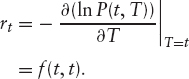
The short rate, r_t, is the instantaneous borrowing rate. It is not observed directly in the market, but can be expressed in term of zero-coupon bonds as

In a short-rate model, the short rate is modeled as some specified stochastic process. For a general single-factor model we will have

where W_t is a Brownian motion in the risk-neutral measure, , where the money market account,

is the numeraire.

Three examples of popular short-rate models are the Hull-White or Vasicek model ([61], [62]):

the Black-Karasinski model ([63]):

and the Cox-Ingersoll-Ross model ([64]):

Each of these models is capable of fitting the entire term structure of interest rates if the yield curve obeys certain constraints. For example, the Black-Karasinski model requires that the forward rate,

is positive for all t. The function θ_t can be calibrated so that the models fit the initial yield curve, that is,

The volatility parameters, σ_t and κ_t, can also be calibrated. While these parameters do affect the fit to the yield curve, they will generally be calibrated to swaption and/or cap prices. For any set of volatility parameters, we must adjust the drift term θ_t to fit the yield curve.

Since we only have a one-factor model, the ways in which the yield curve can evolve are limited, with changes to all forward rates being perfectly correlated. Figure 3.2 shows some possible changes to the forward curve in a simple Hull-White model, whereas figure 3.3 shows actual changes to the forward curve. While one-factor models may capture the dynamics of individual rates, they cannot capture the relationship between different rates. As a consequence, one-factor models are not suitable for pricing derivatives that depend on differences between two market rates, such as CMS spread options.

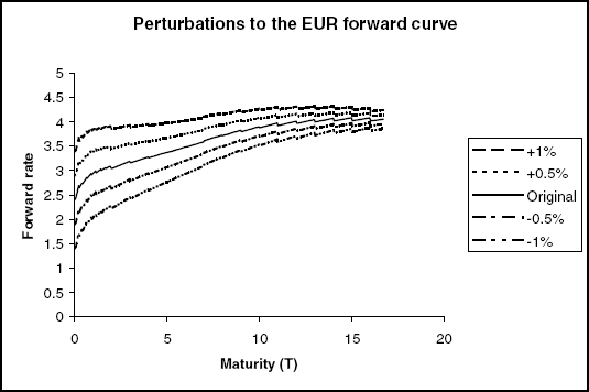
FIGURE 3.2 Possible changes to the forward curve from a single-factor Hull-White model using a mean reversion of 10%. A change to the short rate (the front end of the curve) decays away exponentially with maturity.

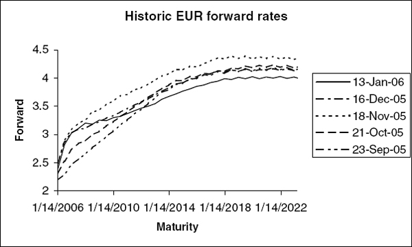
FIGURE 3.3 The EUR forward rate curve calculated from market data on five different dates, shown as a function of maturity.

3.2 ORNSTEIN-UHLENBECK MODELS

We will consider a useful family of short-rate models that can be constructed by expressing the short rate as some function of a variable, x_t, following an Ornstein-Uhlenbeck process:

as

If we let we recover the Hull-White or Vasicek model. If we let we get the Black-Karasinski model (and the Black-Derman-Toy model ([65]) if we set κ = 0). To have more control over the relationship between the short rate and its volatility, we can find some parameterization that interpolates between a normal and a log-normal model, such as

In this model, the limit β = 0 corresponds to the Hull-White or Vasicek model and the limit β = 1 corresponds to the Black-Karasinski model.

3.3 CALIBRATING TO THE YIELD CURVE

3.3.1 Hull-White Model

The Hull-White or Vasicek model is particularly popular as it is the most analytically tractable nontrivial interest rate model. Closed form solutions exist for several options since we have closed forms for both the short-rate distribution and the money market account (our numeraire). In this model we can express the drift θ_t in terms of the initial yield curve P(0, t). However, the expression involves the second derivative of P(0, t), which means we must use some smooth function like a cubic spline for the yield curve. This may not always be ideal as these functions tend to have unwanted nonlocal behavior. However, with a simple change of variables we can remove the need to calculate θ_t and the need to use smooth functions for P(0, t).

As mentioned above, we can rewrite the Hull-White model in terms of some variable x_t whose simple SDE (given by equation (3.2)) does not involve θ_t. We do this by letting

where obeys

Adding this to equation (3.2) recovers the usual Hull-White SDE in equation (3.1). If we choose we have x₀ = 0 and E[x_t|F₀] = 0, so is just the expected future short rate in the risk-neutral measure.

Integrating equation (3.2) we have

where

To show how relates to the yield curve, we need to price a zero-coupon bond:

where

If we let t = 0 and differentiate the log of equation (3.4), we get

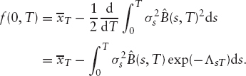
We can use this equation to calculate from the initial yield curve, should we need to. We can also use it to eliminate from the expression for the P(t, T) given in equation (3.4), giving

Since the short rate is not observable in the market, there is no reason why we should explicitly need r_t. Instead, we can use x_t when simulating Monte Carlo paths or writing PDEs for derivatives prices. However, for finding closed-form solutions it is often simpler to work with a slightly different variable,

This has zero expectation in the t−forward measure, We can price derivatives as

for which we need the probability density of in

To calculate the distribution of , we could use the dynamics of x_t in (i.e., equation (3.2)), then change measure to The Radom-Nikodym derivative is just the ratio of the numeraires, so we need an expression for the money market account:

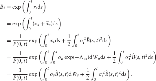
The Radom-Nikodym derivative is therefore

The SDE followed by x under is therefore

with solution

Comparing this to equation (3.6), we see that

To price derivatives in we also need zero-coupon bond prices. Using equation (3.6) to substitute for x_t in equation (3.4) gives

3.3.2 Generic Ornstein-Uhlenbeck Models

In this section we look at fitting the generic short-rate model given in equation (3.3) to the yield curve. Traditionally, this has been done by using forwards induction on trees (see Jamshidian [66] and Hull and White [67]). We present a conceptually very similar approach, using PDEs instead of trees.

Let V(x, t) be the price of a derivative depending on the stochastic interest rates, seen at time t when the parameter governing the short rate is x. Since we are working in the risk-neutral measure, V(x, t)/B_t is a martingale and so

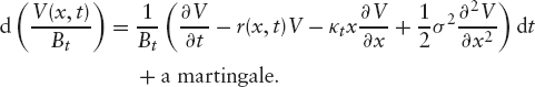
It follows that the price V(x, t) must obey the PDE

Now define the t−forward measure probability density of x as φ(x, t). This must obey

Note that the left-hand side of this equation does not depend on t. This can hold only if φ obeys certain conditions. Differentiating the above equation with respect to t gives

Substituting for using equation (3.8) and integrating by parts gives

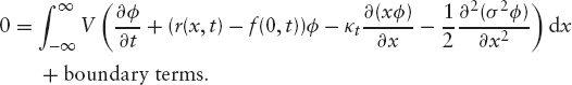
The boundary terms vanish if we assume that φ goes to zero sufficiently quickly as x → ±∞. Since the above equation must hold for any derivative payoff V(x, t), the term in brackets must be zero.⁴ We have the following PDE for φ:

Assuming all of the coefficients of the above equation are well behaved, we can always find some solution φ. However, in order for the model to match the yield curve, we must be able to price zero-coupon bonds correctly. Going back to equation (3.9) and letting V(x, t) = 1 (and so V(x₀, 0) = P(0, t)) we have

Obviously, if this is not satisfied, then φ cannot be the t−forward measure probability density. Differentiating the above equation with respect to t, using equation (3.10) and integrating by parts we get

Again, we have used the properties of φ as x → ±∞ to set the boundary terms to zero. Equations (3.10) and (3.11) together let us fit the model to the yield curve.

Recall that the parameter for fitting the yield curve is embedded in the expression for r(x, t). Going back to our earlier notation, we wrote

so assuming we know φ(x, t) up to some time t, the problem of fitting the model to the yield curve is simply the problem of finding so that equation (3.11) is satisfied.

As an example, in the Hull-White model we wrote

and so we have

which we know to be true since x′ has zero expectation in

We can bootstrap this calibration along since knowledge of φ(x, t) allows us to find , which in turn allows us to find φ(x, t + δt) using some numerical PDE solver.

This simple bootstrapping will give us errors in the propagation from t to t + δt of order (δt)² since we only work out using information at the start of the time-step, and so our approximation for the average in t to t + δt has an error of order δt and we are using it to propagate the PDE a distance δt. However, having done this first step, we then have a solution φ(x, t + δt) that is accurate to O((δt)²) and so we can calculate to order (δt)² and from this get an O((δt)²) solution for the average in the period. We therefore can find φ(x, t + δt) with errors of O(δt³), so after steps, we have an error in φ and of O(δt²).

In figures 3.4 and 3.5, we show the results of fitting a BK model to the EUR yield curve. We used a constant volatility of 10% and a mean reversion of 1%. Note that has discontinuities corresponding to the discontinuities in the forward rate in figure 3.1.

FIGURE 3.4 The probability density (φ) in the BK model using the EUR yield curve, a volatility of 10% and a mean reversion of 1%.

FIGURE 3.5 The integrated drift () for a BK model using the EUR yield curve, a volatility of 10% and a mean reversion of 1%.

3.4 CALIBRATING THE VOLATILITY

In this section we discuss how to calibrate the parameters that govern the volatility structure of short-rate models. In this case, that means the volatility of x and the mean reversion. Mean reversion has the effect of reducing the overall volatility so it must be calibrated alongside the volatility parameters. We will generally want to calibrate the volatility parameters to fit some liquid volatility-dependent instruments such as caps and swaptions.

3.4.1 Hull-White/Vasicek

As before, we will treat the case of the Hull-White/Vasicek model separately as it allows for several closed-form or near-closed-form solutions. In particular, we have closed forms for the zero-coupon bond and the distribution of r_t (see section 3.3.1).

A cap is a string of caplets, which are options to receive LIBOR. We will assume we have dates T_i,0 ≤ i ≤ n, describing n caplet periods. The i’th caplet runs from T_i−1 to T_i, with the LIBOR being fixed (and the exercise decision being made) on date T_i−1 and the payment being received on date T_i. The i’th LIBOR is

where δ_i = T_i−T_i−1 is the day-count fraction for the i’th period. The value of the i’th caplet seen on its exercise date is therefore

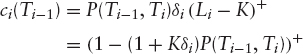
We can now use the results of section 3.3.1 to get a closed-form solution for the price of a caplet. Substituting equation (3.7) into the above equation gives

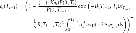
To evaluate this, let so that Z_i is normally distributed with variance Since the exponential is monotonic in Z_i, the caplet will be exercised if

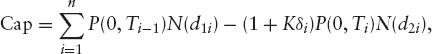
giving a price of

where

The price of the cap is therefore

For pricing swaptions, we can either use a closed-form approximation, or a near-closed-form exact solution. We'll deal with the exact solution first.

A swaption is an option on a swap. We will assume we have an option to pay coupons of K and receive LIBOR. If we also assume the LIBOR fixing, accrual, and payment dates are all aligned, then the i’th LIBOR payment is worth

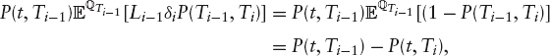
and so the floating side of the swap is worth P(t, T₀) − P(t, T_n). The whole swap is worth

On the exercise date, which we will assume is T₀, the swaption is worth

Substituting for P(T₀, T_i) using equation (3.7) gives

where

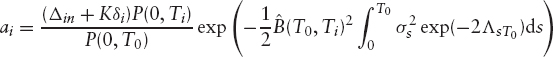
and Δ_in is the Kronecker delta. The swaption is therefore the sum of a series of options on zero-coupon bonds, the strikes being determined by the solution of the equation

As the left-hand side of this equation is clearly monotonically decreasing in x^*, we can solve this very efficiently using a Newton-Raphson method. Once we have found x^*, we can price the swaption as

where F(x^*, t, T) is the price of an option to receive a zero coupon bond P(t, T) at t if that is,

where V_t is the variance of the short-rate distribution at time t,

Alternatively, we can find a closed-form approximation for the swaption price as was first done by Jamshidian [68]. We approximate the sum in equation (3.12) by a single exponential as

If we want to match the expectation of this under the t−forward measure (and thus the price of the swap), we have

We can choose H to match the expectation of the slope of the function. Differentiating both sides of equation (3.13) with respect to x and taking the expectation gives

In figure 3.6, we show an example for a 1y20y swaption with κ = 0.1, σ = 0.1, and zero initial interest rates.

Given this approximation, we can express the swaption price as

FIGURE 3.6 Log-normal swap approximation for a 1y20y swap.

Note that the swaption price depends on σ only up to the exercise date of the swaption. This means that if we fix the mean reversion, we can bootstrap the volatility term-structure. Alternatively, since we can find analytic expressions for the derivatives of the swaption prices with respect to the volatility and mean reversions we could use some Newton-Raphson-based minimization strategy.

3.4.2 Generic Ornstein-Uhlenbeck Models

In this section we discuss calibrating the volatility structure for models that do not have closed-form solutions for swaptions/caps. The important thing is to be able to price caps and swaptions as efficiently as possible. We can use PDE methods to get accurate prices given a set of parameters (kappas, sigmas, and other parameters that the model might have) and then embed the pricing in some minimization algorithm.

Traditionally, we would price a swaption with finite differences by propagating the values of the payments in the swap back to the exercise date, calculating the value of the swaption there, then propagating that price back to the evaluation date. To price an nymy swaption (i.e., a swaption that is exercised after n years into an m year swap) we would have to propagate for n + m years on the PDE grid. However, for each new set of parameters, we must recalibrate , and in doing so we calculate φ(x, t), the probability density of x in the t—forward measure. We therefore do not have to propagate all the way back to the evaluation date, but can propagate the swap price to the exercise date, then use φ to calculate the swaption price with

This reduces the computational cost of pricing the swaption to just propagating m years on the grid.

In the general problem, the price of the nymy swaption depends on the volatility up to the end of the swap (through the drift term ), so it is not possible to bootstrap the volatility. Instead, we have to calibrate the entire volatility term structure simultaneously with some appropriate nonlinear minimization algorithm (see section 3.6).

3.5 PRICING HYBRIDS

In this section we assume we have a stochastic stock process as well as stochastic interest rates. We will model the stock price as

where ν_t incorporates the dividends (assumed to be proportional to the stock price) and the repo rate. We assume the interest rates follow an Ornstein-Uhlenbeck model given by equation (3.3). To distinguish between the stock price process and the interest rate process we will write

We assume we have some correlation structure

Recall that we defined

The volatility of the stock may depend on S_t (i.e., local volatility) or be just a function of time. Calibrating the volatility is the subject of chapter 8, but for now we just mention that the equity process volatility is affected by the interest rate volatility assuming we are calibrating to a market of European options.

We can remove the dividends and repo from the problem by changing variables as follows. Let

We will work in terms of y_t instead of S_t as it is continuous. The analogous SDE to equation (3.14) is

3.5.1 Finite Differences

To find the PDE followed by the prices of the hybrid products we assume we have some derivative whose price depends only on the short-rate driving variable (x_t) and the stock price (or equivalently y_t): V(x, y, t). The value of the derivative discounted by the money market account B_t must be a martingale, so we have

This gives the following PDE for V:

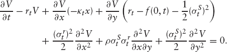
To improve the accuracy slightly, we can work with the deterministically discounted value of the derivative by defining U(x, y, t) = V(x, y, t)P(0, t). This gives the PDE

Unless we represent the yield curve by at least a cubic spline, the forward curve f(0, t) will be discontinuous and so will the short rate r_t. The difference between the two will generally have smaller discontinuities than the short rate itself and is continuous in the Hull-White/Vasicek model and in the limit of zero interest rate volatility. For this reason, U is generally better to work with than V. Note that the PDE for the Vasicek case in terms of r_t involves the drift term θ_t. By writing the PDE in terms of x instead, we have removed the need to calculate this term (which depends on the second derivatives of the zero-coupon bonds). By using U instead of V, we have also removed the need to calculate the forward rate f(0, t) (which depends on the first derivative of the zero-coupon bonds) since r_t − f(0, t) can be expressed in terms of x using equation (3.6) as

We therefore not only do not need twice-differentiable yield curves, or even once-differentiable ones—we can get away with discontinuous forward rates.

3.5.2 Monte Carlo

An alternative method for pricing derivatives is to use Monte Carlo simulation. For that we need to be able to simulate paths of the SDEs followed by x and y. We will treat two cases here—the full problem with local volatility and non-Gaussian interest rates and the special case of the Hull-White/Vasicek model with a term structure of equity volatility; in this case we have a closed form for the Greens function and can therefore take large steps in the simulation.

Vasicek + Term Structure of Log-Normal Equity Volatilities We need to simulate paths of x_t and y_t given by equations (3.2) and (3.15), and the money market account, which follows the process

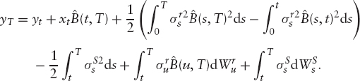
We will consider the changes from t to T. The solution of equation (3.2) is

We can rewrite equation (3.15) as

where is defined in equation 3.5. Using equation (3.17) to substitute for x_T we get

To simulate the money market, we rewrite equation (3.16) as

Once again, we use equation (3.17) to substitute for x_t, giving

In order to simulate the steps from t to T, we must sample from the integrals

We can sample from these if we know the covariance matrix C_ij, where

Let D_ij be the Cholesky decomposition of C, so

If we sample three independent normal variables, Z₁, Z₂, Z₃, we can write

We can therefore simulate paths of the short rate, stock price, and money market account.

Generic Ornstein-Uhlenbeck Models For the more general model given by equations (3.2) and (3.3), we can still simulate x_t exactly, but not the money market account or the stock price. We will therefore have to take small steps in the Monte Carlo simulation where we can find the distribution approximately. Letting T − t = δt, we have the change in the money market account as

The change in the stock variable is given by

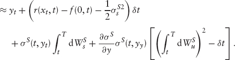
We therefore need to sample from the following stochastic integrals:

with covariances

Overall, this simulation has strong order 1. The interest rate process is simulated exactly and the Milstein scheme we use for the equity process has strong order 1, as does the simulation of the money market account. See Kloeden and Platen [69] for details of Milstein schemes.

3.6 APPENDIX: LEAST-SQUARES MINIMIZATION

When calibrating the parameters of an interest rate model to swaption/cap data, the problem generally reduces to trying to fit m prices by adjusting n parameters. If we have m > n, we cannot necessarily fit all of the prices simultaneously, so we must try to minimize the error in the price in some norm. A commonly chosen norm is the L² norm, where we find the least-square error. If we let the parameters be x = (x₁, x₂,… x_n) and the differences between the market prices and the model prices be y(x) = (y₁, y₂, … y_m)(x), then the problem is to find the vector x that minimizes

While we could use some general algorithm for minimizing a single function of many variables, by reducing the vector y to a single number we throw away useful information about the individual components of y. Many techniques exist for this style of minimization, but here we will just describe two, Newton-Raphson and Broyden's methods, as these are particularly easy to implement. More details can be found in Press et al. [70].

3.6.1 Newton-Raphson Method

When the Jacobian can be calculated simply, such as when calibrating the Hull-White model to swaptions/caps, we can use the Newton-Raphson method to minimize the L² norm. If we have a good trial solution x^k, with residual errors y^k = y(x^k), we can get a better solution by linearizing the problem about this point, giving

We want to minimize

Differentiating with respect to δx and setting the result to zero, we have

The new trial solution is

If we have a linear problem, this technique will solve it in one iteration; for nonlinear problems, the number of iterations will depend on how far away from the linear regime our starting solution is. To handle constraints on the parameters, we can use the sequential quadratic programming method (see [71]) or re-express the original problem in terms of unconstrained parameters. For instance, if we have one original parameter, x, which we know must be strictly positive, we can re-express the problem in terms of x′ = log(x) instead. The new parameter, x′, is free to assume any real value, and ensures that x = exp(x′)> 0.

3.6.2 Broyden's Method

To handle the case where we do not know the derivatives, we can use Broyden's method to estimate them. Here at each step we only have an approximate estimate of the Jacobian

At each step, k, of our iterative procedure, we use the approximate Jacobian to calculate the matrix M and vector v and get the new trial solution x^k+1, then update the estimated Jacobian to be consistent with the previous step. Given that the k’th step is δx^k = x^k+1 − x^k and y changes by δy^k = y^k+1 − y^k, with an estimated Jacobian of B^k, we can compute an updated Jacobian, B^k+1, that satisfies

There is no unique solution to this, but a good thing to use in practice is Broyden's method, where we let

since

For more details, see Press et al. [70].