CHAPTER 2

Applications

While chapter 1 highlighted the principles of equity pricing from a rather theoretical point of view, we want to focus now on practical aspects: we will discuss a few commonly used stochastic volatility models and applications to Cliquet pricing; we will also address the pricing of payoffs that depend on the realized variance of an asset. In particular, “variance swaps” have become very liquid instruments and trading volumes are set to grow even further. The respective options on variance are an attractive new class of products on which to work.

2.1 CLASSIC EQUITY MODELS

In section 1.3.2, we discussed how we can construct martingales that fit a given initial option price surface, the most popular approach being Dupire's implied local volatility. We have already mentioned that in practice, it is rarely possible to obtain a continuum of option prices. Another problem with using an “implied” model is that it does not allow us to control the specific dynamics of the resulting actual stock price process. In this sense, we want to stress that a model that fits very well to some market does not at all guarantee that it produces acceptable prices: for example, consider a stock for which only forwards are traded, but no options. Then a “perfectly fitting” model would be given by a deterministic stock price process.¹ In this case it is obvious that this “model” cannot be correct if we want to price options on the stock. This argument can be carried over to volatility models: The mere fit of a model to European option data does not imply that it gives sensible hedges or prices for exotic payoffs. For this reason, it makes sense to take a “structural” point of view and model the stock and its volatility directly, using a particular assumption on the SDE it satisfies. We will review here a few of such classical stochastic volatility models.

2.1.1 Heston

By far the most popular model is probably Heston's stochastic volatility model [19]. It is given as a solution to the SDE

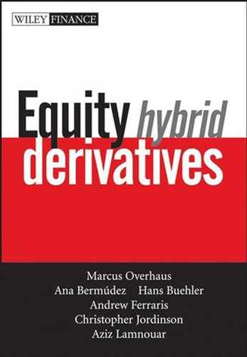
FIGURE 2.1 Stylized effects of changing vol of vol and correlation in Heston's model on the 1y implied volatility. The “Heston” parameters are ζ₀ = 15%², θ = 20%², κ = 1, ρ = 70% and ν = 35%.

where W = (W¹, W²) is a two-dimensional standard Brownian motion. We call κ the “speed of mean reversion” or “mean reversion speed,” the “long vol,” ν the “vol of vol,” ρ the “correlation,” and the initial value the “short vol.” We also refer to θ as “level of mean reversion.” The two parameters vol of vol and correlation can be thought of as being responsible for the skew. This is illustrated in figure 2.1: vol of vol controls the volume of the smile and correlation its “tilt.” A negative correlation produces the desired downward skew of implied volatility. The other three parameters control the term structure of the model:² In figure 2.2, the impact of changing short vol, long vol, and mean reversion speed on the term structure of ATM implied volatility is illustrated. It can be seen that short vol lives up to its name and controls the level of the short dated implied volatilities, while long vol controls the long end. Reversion speed controls the skewness or “decay” of the curve from the short vol level to the long vol level.

Note, however, that the distinction of the parameters by their effect on term structure and strike structure above was made for illustration purposes only: In particular, κ and ν are strongly interdependent if the model is used in the form (2.1). Indeed, κ is meant to be the “speed” of the process, but it does not feature in the volatility term of the variance. This is counterintuitive in the following sense:

FIGURE 2.2 The effects of changing short vol, long vol, and mean-reversion speed on the ATM term structure of implied volatilities. Each graph shows the volatility term structure for 12 years. The reference Heston parameters are ζ₀ = 15%², θ = 20%², κ = 1, ρ = 70% and ν = 35%.

Consider the time change t′ := κt, such that

The process (ζ_t/κ)_t can be seen as being in “unit speed,” κ = 1. From this point of view it would be more natural to parameterize the process ζ in (2.1) as

Properties of Heston's Model One of the most attractive features of Heston's model is the fact that its variance is mean reverting. Such a mean-reverting feature is commonly seen in real market data; see also figure 2.3. Moreover, its calibrated correlation of around −70% is quite stable over time and produces, as we will show, a relatively good fit to the market's implied volatilities, at least for maturities beyond three months. (Figures 2.6, 2.7, and 2.10 show examples of calibrating Heston and other models to market data.)

However, Heston's popularity is probably mainly derived from the fact that it is possible to price European options on X using a semiclosed-form Fourier transformation, which in turn allows rapid calibration of the model parameters to market data.

The underlying mathematical reason for the relative tractability of Heston's model is that ζ is a squared Bessel process, which is well understood and reasonably tractable (cf. Revuz/Yor [13]). In fact, a statistical estimation on SPX by Aït-Sahalia/Kimmel [20] of α ∈ [1/2, 2] in the extended model

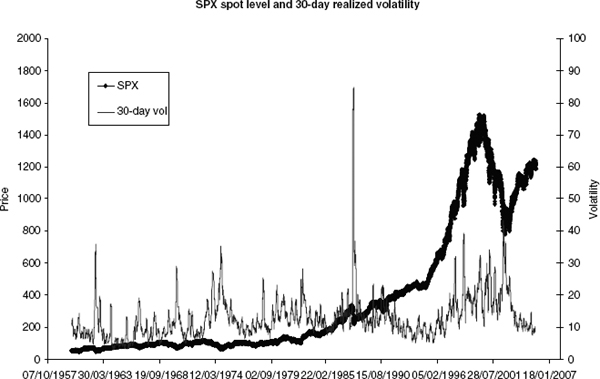
FIGURE 2.3 Historic SPX quotes and estimated 30-day variance. Apart from occasional spikes we can identify the mean-reverting nature of the variance. It should be noted that the level of mean-reversion itself also varies over time.

has shown that, depending on the observation frequency, a value around 0.7 would probably be more adequate. What is more, the square-root volatility term means that unless

the process ζ can reach zero with nonzero probability. The crux is that this conditions is regularly violated if the model is calibrated freely to observed market data. While a vanishing short variance is not a problem in itself (after all, a variance of zero just implies that nobody trades), it makes numerical approximations more complicated. In a Monte Carlo simulation, for example, we have to take the event of ζ being negative into account. The same problem appears in a PDE solver: Heston's PDE becomes degenerate if the short vol hits zero (cf. section 9.4). A violation of (2.3) also implies that the distribution of short variance at some later time t is very wide (see figure 2.4).

Additionally, if (2.3) does not hold, then the stock price X may fail to have a second moment if the correlation is not negative enough in the sense detailed in proposition 3.1 in Andersen/Piterbarg [21]. Again, this is not a problem from a purely mathematical point of view, but it makes numerical schemes less efficient. In particular, Monte Carlo simulations perform much less well. Although an Euler scheme will still converge to the desired value, the speed of convergence deteriorates. Moreover, we cannot safely use control variates anymore if the payoff is not bounded.

Computing European Option Prices with Fourier Transforms To compute European option prices, we focus on the call price. Following Carr/Madan [22], we will price the call via Fourier inversion (see also Lewis [23] for a detailed overview of the subject). Let, as before,

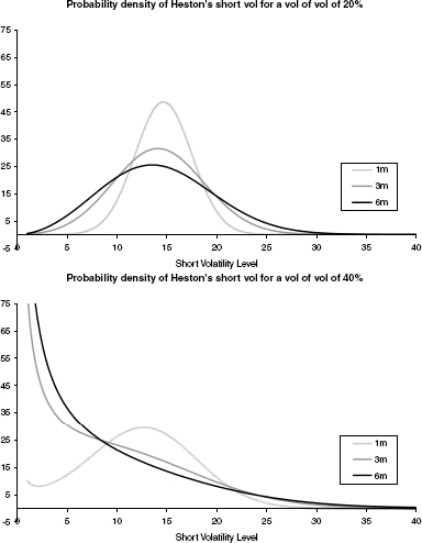
FIGURE 2.4 This graphs shows the density of ζ_t for one, three, and six months for the case where condition (2.3) is satisfied (left side) or not (right side). Apart from the vol of vol, the parameters were ζ₀ = 15%², θ = 20%², and κ = 1.

Since the call price itself is not an L² function in k, we define a dampened call

for an α > 0 (see Carr/Madan [22] for a discussion on the choice of α). We also denote by φ_t the density and by φ_t the characteristic function of log X_t. Then,

We can then price a call on X using

The method also lends itself to Fast-Fourier transformation if a range of option prices for a single maturity is required.

Heston's Characteristic Function Let us now show how we can compute Heston's characteristic function,

We present here an approach that is mathematically not rigorous, but very intuitive. See Heston's original work for a more precise derivation of the characteristic function. We have

where is the complex measure associated with the density We have du for a -Brownian motion B^z. This implies that under , the process ζ satisfies

Here, W^z is a -Brownian motion with a correlation of ρ with respect to B^z. We can therefore compute ψ using the more general function

for a process

To this end, note that because of the Markov property of x, the process (μ, h; x_t) is a martingale on [0, T]. Hence, by using Ito and division by obtain the PDE

with boundary condition η₀(μ, h; x) = e^{−μ x}. Since x is affine, we guess that η is an exponential of an affine function,

By solving the above PDE for this function, we obtain

and

with the constants

For the case where m is time-dependent, see section 2.1.5 below.

Simulating Heston Once we have calibrated the model using the aforementioned semiclosed form solution for the European options, the question is how to evaluate complex products. At our disposal are PDEs and Monte Carlo schemes. We briefly comment on the Monte Carlo approach: we want to simulate the Heston process (2.1) in an interval [0, T]. Since the conditional transition density of the entire process is not known, we have to refrain from solving a discretization of the SDE (2.1). To this end, assume that we are given fixing dates 0 = t₀ < … < t_N = T and let Δt_i := t_i+1 − t_i for i = 0, …, N − 1. Moreover, we denote by ΔW_i for i = 0, …, N − 1 a sequence of independent normal variables with variance Δ_i, and by ΔB_i a corresponding sequence where ΔB_i and ΔW_i have correlation ρ.

When using a straightforward Euler scheme, we will face the problem that ζ can become negative. It works well simply to reduce the volatility term of the variance to the positive part of the variance, that is, to simulate

A flaw of this scheme is that it is biased. This is overcome by using the moment-matching scheme

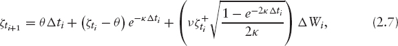
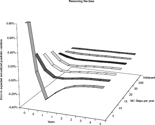
FIGURE 2.5 Plain Euler with various steps per year vs. the unbiased scheme. The model parameters were ζ₀ = 30%², θ = 20%², κ = 2, ρ = −70%, ν = 35%. The graph shows the error between the true and the simulated value of

which works well in practice, see figure 2.5. Higher-order schemes such as Milstein cannot be used with this process since the square root is not differentiable at 0 (this is not such a big problem if we ensure that (2.3) is satisfied). A similar approach is used to compute the stock price: Here, we note that the integral over ζ_t in the interval [t_i, t_i+1] conditional on ζ_ti is given as

hence, we set

A powerful tool to improve the convergence of the estimation of an expectation are control variates (for the case where (2.3) holds). The idea is as follows: Assume we want to compute the expectation of a random variable X (the payoff) and denote by the estimated value of X using n Monte Carlo paths. The standard deviation of the error in this estimate is given by (i.e., it is worthwhile to try to reduce the variance of the variable we estimate). Now assume that there is a second random variable Y (the control variate) whose expectation we know analytically.

The idea is that we estimate the value of X−hY and add back the value of hY. It is clear that this scheme is unbiased if our original Monte Carlo scheme was unbiased. To compute the ideal ρ, note X − hY has the variance Var[X] − 2hVar[X, Y] + h²Var[Y], which is minimized if we set

Since we usually do not know Var[X, Y] and Var[Y], we can replace the above quantities by the estimates on the nth path. Extension of this idea to a number of control variates is straightforward (a good reference on Monte Carlo in practice is Glasserman [17]).

An efficient control variate depends by construction on the actual payoff, but if no other variance reduction techniques are used, using the integrated variance and the stock price is usually a good choice. To this end, we track in addition to ζ and X also V_i+1 := V_i + Δ_iV, which is an unbiased estimator of the integrated variance

2.1.2 SABR

The SABR model introduced by Hagan et al. [24] is given as

for and X₀ = x and α₀ > 0. It is a blend between the CEV model (cf. example 1) and a log-normal volatility model: the former is obtained from (2.8) by using ν = 0, while the latter corresponds to β = 1. This model is very popular in interest rate modeling due to the fact that it is possible to derive approximations for the implied volatility directly from the model parameters. These approximations can then be used to interpolate the implied volatility surface in an arbitrage-free way without the need to compute European option prices numerically with subsequent computation of implied volatilities. The implied volatility for a strike k at maturity T is approximated in [24] as

with

While this model is convenient for marking implied volatilities, it has a few drawbacks when used for pricing equity options. The first issue is that for the case β < 1, the stock price itself becomes zero with a nonzero probability just as the CEV process in example 1. While this might be acceptable for single stocks, this is rarely a desirable feature for index price processes. Another issue is that in the case β = 1 and ρ > 0, the stock price in this model is not a martingale, as Jourdain shows in [25]. He also shows that the model has moments up to order 1/(1 − ρ²); hence, the second moment does not exist for These problems stem from the fact that the model has a log-normal volatility, which implies that volatility can grow exponentially. However, most historic data indicate that an unbounded volatility process is rather unlikely, and that volatility should be mean-reverting in some sense (to this end, see figure 2.3 on page 38). Nonetheless, the model offers an alternative to the Heston model because it can be calibrated very quickly to observed European market prices using (2.9). At the moment, however, it does not seem to beat Heston in terms of fitting the market, as figure 2.6 shows.

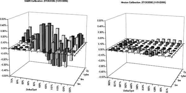
FIGURE 2.6 Calibration of SABR and unconstrained Heston to STOXX50E data for maturities from 3m to 2y. Heston appears to fit better to most indices at the time of writing. The calibrated values were α₀ = 15.9%, ρ = −46.9%, ν = 78.0%, β = 0.58 and X₀ = 0.75 for SABR and v₀ = 15.7%², θ = 40.2%², κ = 0.30, ρ = −68.5% and ν = 38.3% for Heston. The SABR fit is only marginally worse for fixed β = 1 and X₀ = 1, in which case the remaining parameters become α₀ = 15.9%, ρ = −46.9% and ν = 78.0%.

The SABR model has been extended in several ways. In [26] Hagan et al. discuss the model with a more general local volatility function F,

for which they also present analytical approximations. Moreover, Henry-Labordère [27] discusses approximation formulas for much more general models than (2.8). In particular, he introduces a mean-reverting drift into the SDE for α and, additionally, shows how the local volatility function F in the above equations must be chosen to perfectly match the short-end skew. In a recent paper, Bourgade and Croissant [28] also work in this extended framework.

2.1.3 Scott's Exponential Ornstein-Uhlenbeck Model

Scott [29] has proposed a short-variance process, which is modeled as an exponential Ornstein-Uhlenbeck (OU) process,

This process has been investigated in depth by Fouque et al. in [30]. This model shares with the preceding SABR model the loss of the martingale property for ρ > 0 and the limitations if the second moment is to be retained (in fact, Jourdain discusses in [25] both models). From a practical point of view the problem with (2.10) is that no straightforward method is available that allows the efficient computation of European option prices or implied volatilities. It should be noted, however, that the process v itself is very easy to simulate. The complication is to simulate the stock price X, for which we have to revert to solving the SDE (2.10) via discretization. The use of control variates as discussed above improves the convergence of a Monte Carlo scheme, but again this limits us to the case where X has a second moment. However, if we want to price European options, we can make use of the following observation: let ζ_t := e^v_t, then

with

Hence, we have reduced the computation of a European option to a one-factor problem. This obviously works for all “pure” stochastic volatility models where the volatility does not depend functionally on the stock price level.

2.1.4 Other Stochastic Volatility Models

The list of stochastic volatility models that have been proposed for option pricing is long. However, apart from Heston-type and SABR-type models, most stochastic volatility models do not admit an easy access to the pricing of European options or their implied volatilities.³ In contrast, for many Levy models proposed in the literature (see, for example, Overhaus et al. [31] and Shoutens [32]), the characteristic function is available, such that the approach discussed on page 38 can be used to price Europeans. Numerical methods for such models tend to be more involved than for diffusion-based models; see Cont/Tankov [33] for a good account on using Levy models in finance.

2.1.5 Extensions of Heston's Model

Using Heston's model (2.1) as a basis, we can develop a range of related models that still admit a characteristic function that can be computed more or less quickly. The first extension is a model in which the level of mean reversion is time dependent: assume that θ = (θ_t)_t≥0 is a non-negative function and set

A good example, which we will pick up again in section 2.3.3, is θ_t := m + (θ₀ − m)e^−ct. Following the computations for Heston's model, we find that we can still write the characteristic function of log X as an exponential of an affine function as in (2.4). Indeed, the only change is that now, instead of (2.6),

If time dependency of the other parameters of Heston's model is required, we can revert to the case of piecewise constant parameters. Indeed, let us set

with functions κ, θ, ν and ρ, which are piecewise constant on 0 = t₀ < … < t_n. Assume that t_k < T ≤ t_k+1. The characteristic function of log X_T is then given as

for some constants and By iteration, we obtain once again an exponential affine characteristic function of log X_T.

In a different direction, Heston's model can be extended by adding jumps to the return process. A popular example is Bates's “Heston Jump Diffusion” [35], which is a combination of Heston's model and the jump diffusion model with normal jumps in the return as in example 2 on page 20. Since the characteristic function of the jump diffusion part can be computed easily and since the jumps and the Brownian motions are independent, the characteristic function of Bates's model is just the product of the characteristic functions of Heston's model and the Jump Diffusion model with zero short volatility (i.e., σ = 0 in (1.28)). The parameters of this model can also be made time dependent with piecewise constant values.

FIGURE 2.7 Various models fitted to STOXX50E for maturities from 1m to 5y. The introduction of time dependency clearly improves the fit. Figure 2.8 on page 48 shows a summary of the calibration for STOXX50 while figure 2.9 on page 48 and figure 2.10 on page 49 show the summaries for SPX and FTSE, respectively.

When the number of parameters in a model increases, it will usually also fit better to the implied volatility. In particular, the extension (2.11) is a good way of improving the short-end fit of Heston's model to the implied volatility market. If a much better fit is required, the piecewise constant time-dependent Heston model with or without jumps can be used, as is illustrated in figures 2.7 through 2.10.

However, it should be noted that by introducing piecewise constant time-dependent data, we lose much of a model's structure. It is turned from a time-homogeneous model that “takes a view” on the actual evolution of the volatility via its SDE into a kind of an arbitrage-free interpolation of market data: If calibrated without additional constraints to ensure smoothness of the parameters over time, this is reflected in large discrepancies of the parameter values for distinct periods.

FIGURE 2.8 A summary view of the calibration for STOXX50E. The extension of Heston via (2.11) in particular improves the fit of Heston's model to the short end, which is a common problem of the original model.

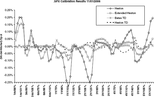
FIGURE 2.9 Calibration results for SPX. The naïve calibration for Heston gives a very bad fit that exceeds the desired 0.10% error threshold frequently.

For example, the excellent fit of the time-dependent Heston model in figure 2.8 is achieved with the following parameter values (short volatility was 15.0%):

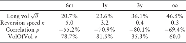
FIGURE 2.10 Calibration results for FTSE.

Moreover, the increased number of parameters makes it more difficult to hedge in such a model in practice. Even though both Heston and the time-dependent Heston models create complete markets, as discussed in section 1.4.1, we will always need to additionally protect our position against moves in the parameters values of our model. Just as for vega in Black and Scholes, this is typically done by computing “parameter greeks” and neutralizing the respective sensitivities. Clearly, the more parameters are involved, and the less stable these are, this “parameter hedge” becomes less and less reliable.

2.1.6 Cliquets

A classic group of “volatility products” in equity markets is called Cliquets. The term generally refers to contracts whose payoff depends one way or the other on the performance of an asset over a future period of time. For example, a globally floored Cliquet with a local floor of 2.5% and a cap of 5% over the reset dates 0 = t₀ < … < t_n = T pays

where we used the notation and Other, more exotic payoffs include:

• Napoleons:

  

• Multiplicative Cliquets:

  

• Reverse Cliquets:

  

  for C > 0 and k > 0.

The evaluation of such products is by far not trivial and the market has not yet settled for an agreed reference model. In fact, at least for single underlying products, a big step forward would be if it were possible to price and, more importantly, actually hedge plain forward-started options consistently. For example, a forward-started call has the payoff

Puts are defined accordingly.⁴

If we want to price a forward-started option of the type above, it is clear that at the reset date t₁, the contract turns into a plain European option. Since such options are liquidly traded, this price must be very accurate. In other words, any model we may propose should internally be able to produce future implied volatility shapes (i.e., European option prices) that are consistent with historic behavior: we have already discussed in section 1.2.1 that the general shape of the implied volatility surface is similar over time. However, we do not necessarily need to fit the entire implied volatility surface perfectly. Intuitively, the main importance is to fit and explain well those implied volatilities at time-to-maturity of the length of the period τ := t_i − t_i−1, so typically one month, three months, six months, or one year.

Stochastic Implied Volatility Under these circumstances, the most natural modeling approach is to model directly the implied volatility surface (or, equivalently, the implied forward distribution or the European option prices). The first such stochastic implied volatility model (to our knowledge) was proposed by Brace et al. in [36].⁵ It has also been discussed by Cont et al. [38] and Haffner [39]. The idea is relatively straightforward: Let us denote by σ_t(T, k) the implied volatility in our model at time t for a strike k and a maturity T. We now want to model this quantity directly as a stochastic process. While it is possible to formulate this idea in terms of stochastic functions in the spirit of Brace et al. [36], we consider here the more direct approach of writing σ in terms of a sufficiently well-behaved function G and an m-dimensional parameter process Z = (Z_t)_t≥0 as

For example, we use a d-dimensional Brownian motion W = (W¹, …, W^d) and assume that the m-dimensional process Z is the unique strong solution to an SDE

for vectors

The function G is chosen such that it gives a reasonable shape of the implied volatility for all possible parameter values This is why we have written G(z; x, c) as a function of the natural coordinates’ time-to-maturity x = T − t and relative strike c = k/X_t instead of fixed maturities and cash strikes. Ideally, the parameters of the process Z would have a direct interpretation such as level, skew, kurtosis, and term structure of the implied volatility surface. However, it should be clear that the specification of such a function and the dynamics of Z are constrained by no-arbitrage conditions: In particular, the price process of each European option should be a local martingale.⁶

The price of a call with cash strike k and maturity T at time t is given by

If the implied volatility surface is well defined, then it follows from the continuity of the stock price process that X is given in the form for some Brownian motion B and with a short variance process ζ, which is the square of the instantaneously maturing implied volatility, ζ_t = σ_t(0; X_t)².⁷ In other words, the call price is a function of X and Z, and as such we can apply Ito. As a result, we obtain a regularity condition on the interplay between , μ, ζ and ζ.

This expression can be expanded using the standard derivatives for the Black & Scholes formula, which results in a complex PDE for ζ and μ (see Brace et al. [36] for details). While this approach is very appealing, it has the unfortunate drawback simply that no “stochastic implied volatility” model has yet been published that is not from the start a stochastic volatility model. The main problem of the entire approach is that it is very difficult to find a function G that actually ensures that the European option prices at any time t are strongly arbitrage free in the sense of definition 1.3.1 on page 16; if a model produces arbitrage situations in itself, then the “price” of a derivative computed with this model is meaningless. Indeed, it seems that the only functional forms for G so far known are those that stem from starting with price process X in the first place: this is one of the motivations of using the SABR model discussed above, for which we have approximative formulas for the implied volatilities. However, even if we use the implied volatility surface function given by, say, a Heston model (2.1) and simply see it as a function

which maps the parameters of the model to an implied volatility surface, the restrictions imposed by the no-arbitrage equation derived above are severe (also see the comments in example 5 on page 75).

REMARK 2.1.1 Instead of modeling implied volatility, we could also consider alternatives such as the call prices on the stock, its implied distribution, or the implied local volatility. The latter has been discussed by Derman/Kani in the related context of their implied trees [40].

2.1.7 Forward-Skew Propagation

To price Cliquets, we have to revert to less ambitious approaches. Note that it is, of course, possible to price a forward-started option using the Black-Scholes formula. For a given flat volatility σ, the price of such a call (2.14) on X is given as

Just as before, this allows us to define what is called the forward implied volatility of a given market price (t₁, t₂, k) for the call as

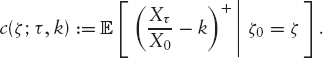
This quantity is often used as a way to quote the price of a forward-started option. For example, we call the forward skew at t₁ for the period τ := t₂ − t₁. Given a particular model, this forward skew can be used to compare the prices of forward-started options with the same reset period τ but with different starting dates: see, for example, the fourth graph in figure 2.12 on page 82, which shows how the forward skew for τ is equal to three-month changes with the start date in a Heston model. We can clearly see that the skew becomes more and more U-shaped.

Sometimes it is required that a model “propagates the skew,” that is, that the forward skew matches the current skew for the same time-to-maturity as closely as possible. One way to achieve this works as follows: As before, denote by τ the period between two reset dates, and we assume that we can extract the distribution of S_t1 from the market using the second derivative in strike of standard spot-started European options. The idea is now to assume that

is independent of Y_j, j = i − 1, …, 1 and that it has exactly the same distribution as Y₁. This implies that the discrete stock price is given as a product of independent variables,

Such a model is called an independent increment model and by construction it will perfectly “preserve the skew.”⁸ Apart from the unrealistic assumption that the increment of a stock price does not depend on its past behavior in any way, this model also has the drawback that the prices of spot-started European options with maturities t₂, …, t_n are completely determined by the initial distribution of Y₁. Consequently, the ATM spot-started options will usually not fit to the market prices. To alleviate this obvious drawback, it has been proposed to maintain the ATM implied volatility for the forward-started options in Black and Scholes and to apply a certain skew to them. These forward starts are then used to back out the assumed distribution of Y_i, which is possible because of the assumption of independent increments: If all forward-started call prices are known, the forward distribution is as usual given by the second derivative of these prices in strike. Hence, a simple model of this type can be realized by jumping independently between the reset dates t_i according to the forward distributions implied by the forward-started call prices.⁹

Blending the Skew Instead of using purely independent increments, it is often desirable to introduce some interdependency between the increments while retaining the possibility of controlling closely the shape of the forward distribution. In fact, what is needed is a model where each Y_i is distributed according to some distribution μ, which is parameterized by a parameter-vector χ. If these parameters are the same for all i = 1, …, n, then the model is an independent increment model.

We want to discuss such a model now: It allows us to blend between a pure independent increment model and a real stochastic volatility model. The idea is to use the distribution in Heston's model for the forward distribution. Using previous results, we can combine the various forward distributions such that it is possible to blend between a pure Heston model and an independent increment model. Let us therefore define for the first interval t ∈ [0, t₁] the initial process

The distribution of X_t1 is then controlled by the parameters To model the next increment, we again want to use Heston's model. Hence, set for t ∈ (t₁, t₂]

The key is that we can introduce a dependency on the values of the previous process by letting

where we usually set to avoid jumps in the forward variance curve of the model. The blending parameter α² allows us to blend from the independent increment case (α² = 1) to the pure (piecewise time-dependent) Heston case (α² = 0). The parameters for the second maturity are χ² = (θ², κ², ρ², ν²; α²). This process can then be iterated to yield a sequence of semidependent short volatilities for each interval. Additionally, the sequence θ¹, …, θⁿ can be used to fit the model to the ATM spot options.

While the other parameters could be chosen freely, it is in the spirit of the approach—propagating the skew—to keep κ, ρ and ν constant, because this implies that the forward distribution of X_ti for i = 2, …, n has the general properties of the initial distribution for X_t1. The parameter α can be varied to assess the impact of co-correlation between the increments. Indeed, if α = 0 and if θ and the start values for each interval, are kept constant, then the model simply is an independent increment model with identically distributed increments.

FIGURE 2.11 The fit of the Heston model to the 3m skew. The calibrated parameters are ζ₀ = 11.25%², θ = 17.39%², κ = 2.75, ρ = −65%, and ν = −51.69% (note that condition (2.3) is violated).

Of course, the general idea of randomizing the parameters of the distribution can be applied to any stock price model, but the “blended Heston skew” model described here has the advantage that the characteristic function of the logarithm of the stock price can be computed easily: in each interval, a formula of the type (2.4) holds. For i = 1, …, n we can find constants Aⁱ and Bⁱ such that

Iteration yields a closed form for the characteristic function. To match the very short-term options better it is possible to add a jump diffusion component along the lines of Bates [35].¹⁰

Example As an example, assume we want to price a Cliquet structure with three monthly reset periods. We have calibrated a Heston model to the following options: 3m calls on 100%, 102.5%, and 105%; 3m puts on 95% and 97.5%; and 1m and 2m calls on 100%. Since the reset period of the Cliquet we want to price is three months, we have given the 3m options twice as much weight as the other two options.

The resulting Heston model fits very well to the calibration instruments, as shown in figure 2.11.

As a next step, we have set up the above model with θⁱ := θ, νⁱ = ν, ρⁱ = ρ and for i = 1, …, n. As a result, the model is just the calibrated Heston model as long as αⁱ = 0, while it is an independent increment model if we set αⁱ = 1; note that the increments are not exactly identically distributed because the short vol parameters vary. The interesting point is now the impact on the forward skew of changing α between these extreme values: Figure 2.12 shows how α blends between a skew-preserving model and a true homogeneous Markovian model.

Finally, we can assess the impact of the blending of the skew when pricing a Cliquet structure. As an example, we show in figure 2.13 what happens when we price the globally floored Cliquet (2.13).

REMARK 2.1.2 The last graph of figure 2.12 shows the usual effect that in stochastic volatility models the forward skew for start dates that are farther away tends to become more “U-shaped.” The reason for this behavior can be explained as follows: For a time-homogeneous stochastic volatility model such as Heston, the price of a forward-started call on X with reset date t₁, maturity t₂, and strike k is given as

with

At time t₁, the implied volatility for the relative strike k and time-to-maturity τ := t₂ − t₁ is according to (1.22) given as

that is, it is a function of the random short variance ζ_t1. Due to the homogeneity of the model, the skew will be very similar in shape to for all reasonable values of ζ_t1. In particular, the “expected future skew” is nearly the same as (see figure 2.14). The quantity “forward skew,” on the other hand, is given as

Since is concave for out-of-the-money options, it follows from Jensen that we obtain the observed U-shape. It seems theoretically more natural to preserve the expected future skew instead of the forward skew. The former is a genuine property of all homogeneous stochastic volatility models.

2.2 VARIANCE SWAPS, ENTROPY SWAPS, GAMMA SWAPS

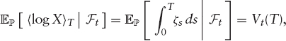
We have seen that under the assumption that sufficiently many European options on the underlying S, or X, are traded, we can price European payoffs uniquely using (1.29) or its discrete version (1.30). A particularly popular application of (1.29) is the pricing of variance swaps, suggested first by Neuberger. We also present two relatively new products, entropy swaps and gamma swaps.

FIGURE 2.12 The impact of changing the blending parameter α on the forward skew. We can clearly see the usual increasingly upward-sloping forward skew in the classic Heston model.

FIGURE 2.13 The price of the globally floored Cliquet (2.13) with maturity in two years along with the values of the prices of the involved forward-started call spreads. The price differences stem mostly from the difference in the prices of the forward-started options, rather than the global floor.

FIGURE 2.14 Forward skew and expected future skew in the Heston model.

2.2.1 Variance Swaps

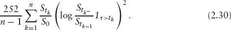
A variance swap with maturity T is a contract that pays the realized variance of the return of the stock over the period [0, T] in exchange for a previously agreed strike, K² (the strike is usually quoted in “volatility,” K). In the absence of any proportional or fixed dividends, and no risk of default, the realized variance is commonly defined as

where 0 = t₀ < … < t_n := T are the business days in the period [0, T]. The scaling factor

“annualizes” the returned variance: the number 252 is the standardized number of business days per year; we can think of [T] as being approximately T. If the stock price pays dividends and is subject to default risk, then we use here

where denotes the discrete cash dividend paid at t_k and where proportional dividend for this date, cf. (1.10). The idea of this convention is that we do not want to count movements of the stock price that are due to (previously known) dividend payments. Indeed, if no further dividends are paid in (t_k−1, t_k), we obtain (cf. equation (1.6) on page 7):

In practice, default risk is not excluded as in (2.16), but by imposing a cap on the overall realized variance (discussed on page 64 ff). Moreover, dividends are in practice taken out only for single stocks; for indices, (2.15) is used. See remark 2.2.1 for the impact of dividends. Let us first consider the case where dividends are taken out (i.e., (2.16)).

Given dividend dates 0 = τ₀ < … < τ_m = T, we have

We will assume that the right-hand side is in fact the definition of realized variance (cf. remark 2.2.1 below). A variance swap pays the actual realized variance up to its maturity T in exchange for a previously agreed strike K². Its payoff is therefore

We will denote by the value at time t of a variance swap with strike K and maturity T. Since both and K are constants, it is sufficient to compute the expectation (2.17) for the purpose of evaluating a variance swap, which is given by

If is a pricing measure, and if there are no cash dividends, this means that

The fair strike K*(T) for this maturity, which renders the initial value of the trade zero, is therefore

REMARK 2.2.1 Note that approximation (2.17) works well if we want to price variance swaps. However, the pathwise approximation of realized variance by quadratic variation is not perfect, as is illustrated in figure 2.15. This is particularly important if we price nonaffine payoffs of realized variance; see Barnorff-Nielsen et al. [41] for a discussion on the properties of the error.

FIGURE 2.15 The quality of the approximation of realized variance by quadratic variation. The graph shows an example path of each of the two quantities for Heston's model with the calibrated parameters from figure 2.6.

Pricing and Hedging Following Demeterfi et al. [42], we henceforth assume that the pure stock price X is continuous, and that is absolutely continuous with respect to the Lebesgue measure. We have mentioned already in section 1.1.2 that this implies that there exists a stochastic short variance process ζ = (ζ_t)_t≥0 and a Brownian motion B such that

where denotes again the Doleans-Dade-exponential. Accordingly, the quadratic variation of the returns of X is given as

On [τ_j−1, τ_j) with τ > τ_j, we have Hence,¹¹

Hence,

Let us focus for a moment on the case when there are no discrete cash dividends. We obtain

and, using

This means that we can replicate realized variance by holding a static position in a log-contract with payoff −2 log S_T and by dynamic delta-hedging with a delta of Δ_t := 2/S_t− (for clarity of exposure we ignore discounting here). One particular point is that the cash-delta (2.19) is constant: we hold at all times the value 2 in the stock. Similarly, the gamma implies that our cash gamma of is constant, too. (In the light of the discussion below this makes a variance swap particularly suited to “trade volatility.”) For (2.18), the expression is slightly more complicated, but it is still of the same basic structure. (Note that additional terms are European-type payoffs on S, whose value can be computed using formula (1.29).)

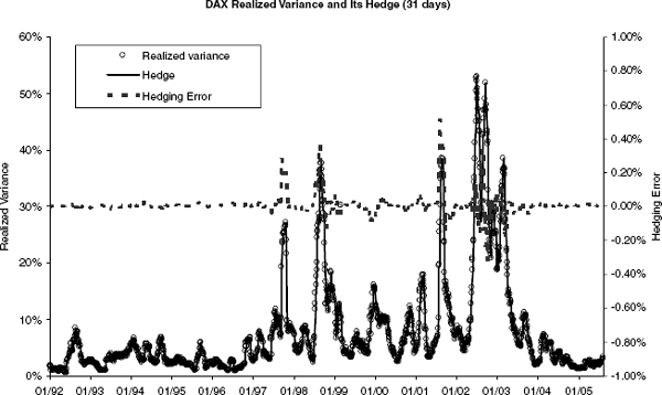
FIGURE 2.16 The quality of hedging variance swaps with (2.19). The graph shows daily the realized variance over 31 business days, the return from the hedging strategy (2.19), and the hedging error.

To assess the quality of the hedging strategy implied by this equation, we have used historic DAX returns and priced a variance swap against two log-contracts plus their daily delta-hedge. Figure 2.16 shows the impressive performance of this hedge.

To calculate the cost of exercising this strategy, note that under any equivalent matringale , the expectation of the right hand side of (2.19) is given as

To compute , note that this value is equal to with H (x) = x − 1 − log x, the function shown in figure 1.6 on page 23.

This function can also be used to center the strip of options around some “reference strike” To this end, note that has a minimum of zero in We have

that is,

Following this strategy, that is, taking a static position in instead of − log S_T, requires an additional position in a future. See Demeterfi et al. [42] for an extensive discussion of this subject. Also, Carr/Madan discuss various extensions of the idea of pricing volatility-sensitive options via hedging arguments similar to (2.21) in [43]. For example, it can be shown that pricing H via (1.31) means that in actual fact, a corridor variance swap is priced, that is, the returns in the sum (2.16) will be counted only if the stock price is between the lowest and highest strike of (2.21). Therefore, a sufficiently wide strike range should be used. Corridor variance swaps and their hedging are discussed in Carr/Lewis [44].

REMARK 2.2.2 In some contracts, in particular for indices, realized variance is defined using equation (2.15), even if dividends are present. In that case, we have to evaluate

The additional terms (of which there are only finitely many) can be hedged and priced with European options using formula (1.29).

Trading Volatility Apart from the fact that variance swaps can be hedged and priced using European options and a clearly defined delta-hedging strategy, what are the reasons to trade this product?

One motivation to trade in volatility is that apart from the stock, the price of an equity derivative is massively dependent on the volatility of the stock price. Practitioners therefore seek to protect themselves against moves in volatility. A very common method works as follows (assume that X = S): To price an option with payoff H(X_T), we use the Black-Scholes model with a constant volatility σ,

where we estimate a reasonable σ from European options traded at maturity T. For example, we might decide that the payoff H is sufficiently close to a call with maturity T and strike k with a market price of ₀(T, k) at time zero. Its implied volatility (cf. definition 1.2.1) is denoted by , and we choose to use this implied volatility for our Black-Scholes model (2.22) by setting Let us to denote the real market price process.

Then, our price for H is given as

At some later time t, the value of H given the observed spot is then computed as

That works well if the real price process is a Black-Scholes diffusion with volatility σ. In reality, though, that is unlikely. Assume, for example, that in fact

for some stochastic short variance ζ = (ζ_t)_t≥0. Then, our price (2.23) evolves as

Using the fact that h is a Black-Scholes price for H and that it therefore satisfies the Black-Scholes PDE

we have

(See also the results from El Karoui, Jeanblanc-Picquè and Shreve [45].) The cost of our strategy to replicate H(X_T) via its Black-Scholes hedge is therefore not covered by the initial price The term

shows that we will have an additional contribution from the mismatch in volatility weighted by cash gamma ¹² For convex payoffs, cash gamma will be positive, so we see that we lose money if the real variance ζ stays above σ, and we will gain if our initial guess was larger than the real variance. Equation (2.25) also reveals that it is not sufficient for a perfect hedge that the realized variance, equals σ²T.

Vega Hedging To protect ourselves against the profit and loss swings arising from a wrong volatility assumption in (2.25), it is natural to readjust the Black-Scholes volatility during the life of the product. After all, if we price the call (T, k) itself, we will not match the market as soon as its implied volatility changes.

Assume therefore that at some later time t, the call trades at some _t ≡ _t(T, K). We can then infer its implied volatility by inverting the Black-Scholes price for the call,¹³

Hence, the our price process for H is now given as

A common practice is to protect the position against the change in volatility by vega hedging. The idea is to buy as many calls _t such that the overall sensitivity of the position to changes in both and is zero (recall that the derivative of a price with respect to volatility is called vega; hence the name vega hedging). In our case, this means first to define the Black-Scholes delta-neutral portfolio

and then build a hedging position

The first observation is that this strategy applied to the payoff H(X_T) := (X_T − k)⁺ will yield a perfect hedge: we simply hold . This is an advantage over the pure delta-hedging strategy discussed initially.

However, it is clear that we still do not cover the cost of this hedge with our initial price, . Heuristically, we expect that the hedge above works better, but it is not clear that this is actually true in practice. Another problem with this approach is that it requires us, at least in this pure form, to select a reference option that can be used for vega hedging. In light of today's strong volatility skews, the choice of a strike is a tricky problem and requires a good knowledge of the product that we want to risk manage.¹⁴

Here is where the variance swaps come in: Their price does not depend on a strike. Moreover, their payoff is directly the realized variance; hence, variance swaps are a more natural instrument to hedge against changes in volatility. Indeed, variance swap trades are in practice quoted in units of vega.

The idea behind trading vega is as follows: In terms of the variance swap volatility σ := K*(T), a variance swap with maturity T pays out the quantity σ².

This payoff has a vega of

If we now assume that we have an overall vega exposure ν in our trading book, we can neutralize this exposure by buying

units of variance swaps (the quantity N is the “notional” of a trade of ν). This approach is consistent with the idea of hedging volatility exposure with variance swaps. (For a thorough account on this approach, see section 2.3). However, it requires that the vega of the portfolio is the sensitivity of the portfolio with respect to changes in the fair strike of the variance swap. In particular, it requires us to compute all option payoffs with a model that at least reprices the Europeans in (1.30) and therefore the variance swap itself.

More commonly, though, the vega of a book is an accumulated sum of Black-Scholes vegas across strikes (and possibly maturities), as discussed above. In this case, it seems sensible to assign the Black-Scholes vegas per strike weights according to (1.30). Of course, such an approach does not generally produce a perfect hedge, and it also disrespects changes in skew and kurtosis of the implied volatility surface.

Volatility as an Asset Class Apart from the potential use of variance swaps for vega hedging, they also offer the investor a way to invest in volatility. This can be attractive for many reasons. One of the most interesting properties is that volatility tends to be anticorrelated to movements of the market. Volatility increases if the market is falling and often decreases if the market rallies. (Note, though, that during the dotcom boom both price levels and volatility rose; cf. figure 2.3.) Now, most market participants would probably prefer to trade implied volatility in some way.

The drawback of using plain implied volatility as an underlying, however, is that once a strike of the respective option, to which the implied volatility refers, is fixed (for example at-the-money), this strike can entirely change its characteristics depending on the movements of the stock price. For example, if we start off with a strike at-the-money and the market starts to fall, we end up with an out-of-the money strike above current spot level. Implied volatility in this region often appears to be “cheap.” (For most indices, upside implied volatility is lower than at-the-money implied volatility.) Moreover, the farther out the strike, the less liquid the corresponding option becomes, with the effect of increasing transaction costs.

Here, variance swaps are a good and relatively inexpensive alternative (in terms of transaction costs). They offer exposure to volatility in a way that does not depend on the level of the market in the sense above. Indeed, cash gamma of a variance swap is simply constant 2, if we use the static replication strategy (2.21). In fact, we could also define the variance as the contract that has a constant cash gamma, that is, as the contract that always has the same sensitivity to changes in realized variance, regardless of the level of the stock. See Demeterfi et al. [42] for this approach. A linear cash gamma can be realized using gamma swaps, which are discussed below.

REMARK 2.2.3 The market's interest in trading volatility has led to the introduction of “variance indices,” notably VIX for SPX and VDAX for the GDAXI. These indices can be seen as rolling the square-root of variance swaps with a fixed maturity, a property that makes them very costly to replicate.

It is also noteworthy that trading in options on VIX futures started on CBOE in February 2006.

As soon as trading in variance swaps began, it became clear that variance swaps on single names are very sensitive to large price moves in the underlying asset, as can be seen easily from equation (2.15). In particular, the payout will be infinite if the asset defaults (recall that in practice, the case of default is not excluded by using definition (2.16)). For this reason, investors who sold variance swaps have requested to impose a cap on the potential payout of a variance swap. Typically, this cap is around 250% of K²; that is, the payoff of such a capped variance swap is, in the absence of dividends,

This is equivalent to

The latter payoff is also valid in the presence of dividends if (2.16) is used plus the additional payoff of 250%K² in the event of default.

By requesting protection against extreme stock price movements, investors who sold the capped variance swaps essentially bought out-of-the-money calls on variance. The availability of such products then spurred the development of more standard options: common options on variance that are available today are simple calls

and puts

but also volatility swaps with payoff

(Note that value of a zero-strike volatility swap is always less than the value of a zero-strike variance swap.) More recently, options on forward variance swaps have emerged. For example, a call on forward variance between T₁ and T₂ has at time T₁ the payoff

where V_t(T₁, T₂) is the price at time t of the variance between T₁ and T₂, that is,

It should be noted that this contract has a different nature than a forward starting call on variance swap, which pays at T₂ the quantity

where k is now a relative strike.

REMARK 2.2.4 (Quoting Conventions) European options on variance such as (2.27) and (2.28) are usually quoted in terms of “vol points,”

As before, K*(T) denotes the variance swap volatility.

2.2.2 Entropy Swaps

Since variance swaps offer exposure to the realized volatility of the returns of the stock X, they are relatively insensitive to the level of the stock price.¹⁵ As an alternative measure of variance, it is possible to define the payoff of what we will call an entropy swap as

Intuitively, this “entropy variance” has the convenient property that if stock price and short variance are negatively correlated, then rises in one quantity are offset by falls of the other. Moreover, if the market drifts sidewards (i.e., the level of X does not change much), then the payoff behaves roughly like a variance swap: If the instantaneous correlation between X and ζ is zero, then the value of weighted variance and standard variance are equal. Price and hedging strategy of such a swap can be computed using the same ideas as above. To this end, note that

Hence, pricing an entropy swap boils down to approximate the convex and bounded function H(x) := x log x − x + 1 via (1.29); while the weights for evaluating a variance swap via (1.29) are given as 1/k², they are 1/k in the case of an entropy swap. Since X is a martingale with X₀ = 1, we can compute the value of an entropy swap with maturity T at time 0 as

Let us define the stock price measure by setting for all A ∈ F_T and all T < ∞. This measure is given by using X itself as a numeraire, and the above expression shows that is simply the relative entropy of with respect to , hence the name entropy swap.

Shadow Options The connection between an entropy swap and the measure goes further: we have

In other words, the price of an entropy swap is the value of a variance swap under . With regard to this measure, recall that we used U(T, k) to denote a put on X with strike k and maturity T. Hence,

where we call C^X following Lewis [23] the “shadow call” on X. It is the call on under the numeraire X. The shadow put u^X is defined similarly; together we have

Hence, the shadow option prices can be read from the market. So, in principle, we could compute the value of an entropy swap, using (1.29) in terms of shadow options.

2.2.3 Gamma Swaps

While entropy swaps are an interesting alternative to variance swaps, they are not particularly well suited for real-life investments, because they require us to strip dividends, repo, and interest rates from the traded stock price, S, in order to obtain X. This is very unnatural from an economic point of view and inconveniences the investor. This drawback can be overcome by using what are called gamma swaps or weighted variance swaps: A gamma swap pays at maturity the weighted variance of the stock price,

Assuming that there are no cash dividends, we approximate (2.30) as

A gamma swap has the same attractive property as the entropy swap of being exposed to correlation between stock price and volatility. See figure 2.17 for past performance of gamma swaps. Under the assumption of continuity of X, the price of a gamma swap is

FIGURE 2.17 Past performance of 1y variance and gamma swaps on STOXX50E. We have also plotted the return performance of the index.

(recall the symbols and A_t from page 7). In other words, a gamma swap is a sequence of forward variance swaps and forward entropy swaps. We can approximate its price as

When it comes to hedging a gamma swap, let h ≡ 0 and define H(x) := x log x − x + 1 as above. Let us also recall equation (1.12) and Ito's formula (1.13). They give us again a hedging program,

similar to (2.19). Here, we can see why the product is called gamma swap: The cash gamma for this product is (i.e., linear in spot). The performance of this hedge for real-life gamma swaps is as good as it is for variance swaps, as figure 2.18 shows.

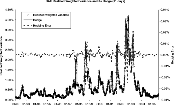
FIGURE 2.18 The quality of hedging weighted variance swaps with (2.31). The graph shows the daily realized weighted variance over 31 business days, the return from the hedging strategy (2.19), and the hedging error.

2.3 VARIANCE SWAP MARKET MODELS

While the evaluation of variance swaps, entropy swaps and gamma swaps is relatively model independent, such formulas are not known for options on realized variance, as introduced in section 2.2.1.¹⁶ To price and hedge a call (2.27) on realized variance on a stock where only European options are traded, we have to use a particular stock price model. In this section we will discuss a general modeling approach that is based on the idea to hedge options on variance with variance swaps. As an illustration, figure 2.19 shows the term structure of variance swap fair strikes K^* for a few major indices. The aim is to model the entire curve of variance swaps as a random variable and then derive in a second step the dynamics of a stock price process that realizes the modeled variance. (We do not attempt to develop a model that prices variance swaps; rather, their prices are input parameters for the model.) Of course, a model that describes well the evolution of variance swap price curves cannot only be used to hedge options on realized variance. Since we will also provide an “associated stock price process” in the model (and an intuitive meaning of correlation), we can use such a model to price and hedge any exotic derivative. For example, it is natural to hedge Cliquet-type products as discussed in section 2.1.6 using forward started variance swaps.¹⁷ This approach is particularly appealing in the light of recent trading volumes in variance swaps.

FIGURE 2.19 Variance swap fair strikes for major stock price markets.

The entire approach is very similar to the Heath-Jarrow-Merton (HJM) approach [47] in interest rates. There, the dynamics of the forward interest rates are modeled as stochastic variables; we will consider forward variance. The basic assumption is that alongside the “pure” stock X, at any time t, (zero-strike) variance swaps for all finite maturities with prices

are liquidly traded. Under the assumption of “no free lunch with vanishing risk,” there exists an equivalent measure under which both X and all variance swap price processes and therefore V = (VT))_T≥0 are local martingales (for ease of exposure we will frequently refer to V(T) as the price process of a variance swap even though, strictly speaking, the price process is V(T)/[T]). While variance swap prices V are readily available in the market, they are slightly difficult to model directly: Since the prices V_t = (V_t(T))_T≥t of variance swaps have to be increasing in T at any time t, it is more natural to work instead with the forward variances

Forward variance is “the market's expectation” at time t of the variance at time T, just as the forward rate in interest rates is the expectation of the short interest rate under the forward measure. (Note that in contrast to a forward rate, a forward variance of zero is a natural state, for example, on weekends.) The main point is that due to its definition (2.32), forward variance itself is tradable and must therefore be a local martingale under a pricing measure, if such a measure exists.

As with interest rates, it is much more natural to look at the evolution of the forward variance curve over time in “fixed time-to-maturity,” rather than a fixed maturity. We expect the properties of forward variance v_t(T) to change markedly during the remaining time to maturity T − t: for example, very long-term forward variance should not be as volatile as short-term forward variance. It is therefore more convenient to use the Musiela parametrization¹⁸ of forward variance,

Accordingly, the price of a variance swap (modulo scaling by the inverse of time-to-maturity) in Musiela-parametrization is

HJM Theory for Variance Swaps The idea of “variance curve models” as introduced by Buehler [49] is now to start by specifying the dynamics of the family u = (u(x))_x≥0 itself, just as HJM-type interest rate models are specified by starting with the forward rate dynamics. The additional complication in the case of forward variance is that we do not only want to model the variance swap prices in this way, but we also need to model a consistent stock price process whose expected realized variance is the price of the respective variance swap. We ignore the effects of dividends in this section.

To formalize our setup, assume that we have a d-dimensional Brownian motion W = (W¹, …, W^d) under a measure , which creates the filtration We will model the variance curves directly under their martingale measure; the ideas from section 1.4 will then be used to derive conditions on market completeness. Assume that u = (u(x))_x≥0 is a family of non-negative processes u(x) = (u_t(x))_t≥0 given by

for some integrable predictable processes α and β = (β¹, …, β^d). Reversing the construction above, we can then define the forward variance processes v = (v(T))_T≥0 by setting

(note that v_t(T) is well-defined for t > T). Equivalently, the variance swap price processes for finite maturities T are defined as

DEFINITION 2.3.1 We call u given by (2.34) a variance curve model if v(T) given by (2.35) is a local martingale for all T < ∞ and if there exists a local martingale X for the stock price such that

for all t and all T < ∞.

Let us assess when a curve u is indeed a variance curve model.¹⁹ First of all, it is natural to assume that all initial variance swap prices are finite, that is,

for all x < ∞. Indeed, if this does not hold, the expected value of the logarithm of X cannot exist. Second, we have to ensure that for each T < ∞, the process v(T) is a local martingale. To this end, we require that β is in C¹ and its derivative ∂_xβ(x) is integrable with respect to Brownian motion. Then,

which implies that the following HJM drift condition for forward variance must hold:

As a next step, note that the process

is an adapted non-negative process. Since its square root is integrable with respect to any Brownian motion B. Each such Brownian motion B can be written in terms of W as

where ρ = (ρ¹, …, ρ^d) is some potentially stochastic “correlation vector” with values in [−1, +1]^d, which always has unit norm, This means that

is a well-defined local martingale with the property that

just as required. We call X an associated stock price process to u.

The Brownian motion B or, alternatively, the correlation vector ρ was arbitrary in the construction of X. Indeed, B plays the role of a “correlation” or “skew” parameter: If the dynamics of u in the form of β are given, then the specification of ρ links the movement of the variance curve with the stock price movement. In particular, this implies that volatility structure of the variance curve and its correlation with the stock price movement can be estimated one after the other.

However, the general formulation of a variance curve above in terms of equation (2.34) plus the requirement of non-negativity is more subtle than it may appear in the first place. Indeed, it is very difficult to assess whether a general stochastic integral (2.34) will remain non-negative. In particular it means that we cannot—as in the HJM-framework for interest rates—specify the volatility structure β independently of the initially observed forward variance curve u₀.

A natural approach to this problem is to model u as an exponential,

where w satisfies the integral equation

Applying our previous results implies the HJM-type drift condition

This approach is well suited for statistical estimation of a volatility structure independent of the initial state u₀ of the variance curve, for example, via a PCA-type estimation of the factors driving the curve. However, it should be noted that this approach also excludes all those classical stochastic volatility models that allow the volatility to reach zero, such as Heston's. Moreover, it is usually more complicated to ensure a true martingale property for the process X if u is given in the form above: recall in particular Jourdain's results [25] for the SABR model and for Scott's model, which we discussed in sections 2.1.2 and 2.1.3, respectively. Nonetheless, given a “volatility structure” w that ensures the martingale property for all initial values u, the above formulation can be used to “fit the market.” This will be discussed in section 2.3.3.

2.3.1 Finite Dimensional Parametrizations

One drawback of our approach so far is that we formulated the dynamics for u in a very general way. But in practice, the formulation of u in terms of a predictable integral equation (2.34) is inconvenient for numerical purposes. Moreover, this formulation implies that the entire curve u is the state of the process, an object difficult to handle on a computer. What we are really interested in is a finite-dimensional representation of the curve u. Indeed, in real life, a finite number of variance swap market quotes is usually interpolated or approximated by some nonnegative increasing functional , which itself depends on only a finite number of parameters If Z_t is the parameter vector at time t, this means that the price at time t of a variance swap starting in t with time-to-maturity x is given as

Since the function must be increasing in x, we can set such that the forward variance process is given as

The process Z = (Z_t)_t≥0 is called the parameter process of the functional G. The idea is to restrict the dynamics of Z to ensure that the forward variances v_t(T) = G(Z_t; T − t) are local martingales.

To this end, recall the definition of the driving diffusion in section 1.4, equation (1.40). There, we have assumed that the entire market of tradable instruments has been given as a functional of a finite-dimensional diffusion (Z⁰, …, Z^m) where Z⁰ represented the stock price X itself. We have shown that such a framework is naturally complete in the sense that “delta hedging works” if assumption 1 on page 32 holds. Consequently, we will use the last m parameters Z = (Z¹, …, Z^m) to drive the parameters of the function G, and incorporate the associated stock price X = Z⁰ afterwards. To this end, assume that on the open set the SDE

for a drift vector and volatility vectors ζ = (ζ¹, …, ζ^d) with has a unique, strong solution. Moreover, assume that the variance curve functional is a C^2,2 function with finite variance swap prices for all states i.e. for all T < ∞. A direct application of Ito shows that the family u defined by (2.38) is a variance curve model if, and only if, the “consistency condition”

holds for all and if ν(T) is a true martingale for all finite T.²⁰

REMARK 2.3.1 It should be noted that we look at the heat equation (2.39) here in a nonclassical way: obviously, if the process Z is given, then (2.39) is satisfied for all functions G defined as in terms of a suitably well-behaved function g.

In contrast, here we start with the function G and ask when a process Z exists to satisfy (2.39): The idea is that we observe the variance swap market data and then choose a suitable function G, which interpolates these data well. Afterwards we use (2.39) to derive constraints on the dynamics on the parameters that drive the curve to ensure that the resulting variance swap price processes are local martingales. The entire approach is very closely related to the idea of a “finite dimensional parametrization” of a variance curve, cf. [49]. This concept has been developed in the context of interest rate theory by Björk/Svensson [51], Filipovic [52] and Filipovic/Teichmann [53].

The Associated Stock Price Once we have obtained what we call a consistent pair (G, Z), the next step is again to construct an associated stock price process X. From the considerations of the previous section, we know that the short variance of X is given by u_t(0) = G(Z_t; 0). It remains to model an appropriate correlation structure; to this end, assume that ρ = (ρ¹, …, ρ^d) is a “local” correlation vector; that is, ρ^j for j = 1, …, d is a measurable function such that for all (z, s). Then, the stock price X is the strong unique solution to

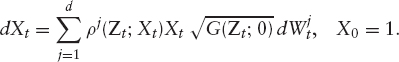
The solution exists and is unique because ρ^j(Z_t; x)x is process Lipschitz for all j = 1, …, d, hence is a well-defined non-negative local martingale, and we call the triplet (G, Z, ρ) a variance curve market model. It models all relevant market instruments jointly in an arbitrage-free way. This setting also includes local volatility models (in which case X itself is part of the vector Z) and, naturally, stochastic volatility models. Moreover, the current framework fits into the settings of section 1.4: The vector is Markov by construction; the market instruments are the stock X itself and the variance swaps with price processes

The process with dV_t(t) = G(Z_t; 0) dt represents the running variance of log X. Without loss of generality we can assume that Let us then define variance swap price functional

which gives the price of a variance swap with maturity T > t in terms of Z as If this functional can be inverted locally in the sense that there is some ε > 0 and some time-to-maturities x_M > … x₁ > ε such that the function

is invertible for 0 < t < ∈, then it is possible to extract locally the vector Z_t from the observation of only V_t(t) and a finite number of variance swaps with maturities T_i = x_i + t. If this function and therefore also its inverse is C¹, then the results of section 1.4 can be applied, which means that under assumption 1 the market given by (G, Z, ρ) is complete. Moreover, all the payoffs depending on the value processes of X and the variance swaps can be replicated by trading in stock and variance swaps (see Buehler [54] for technical details).

REMARK 2.3.2 (Delta in Stochastic Volatility Models) In the particular case where the correlation vector ρ does not depend on X, the stock price at some later time T depends on the current level X_t only through its initial value. This allows us to compute the delta of a European option directly from market data without the need to calibrate a model: We can write the price of a call with maturity T and strike k as

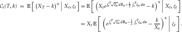
Hence, the “stochastic volatility delta” for any model that is well fitted to the market is given as

That implies, in particular, that two different stochastic volatility models of this type that fit the market prices perfectly will have the same delta. Hence, the only way “pure” two-factor models can be distinguished is via their “vega hedge.”²¹

It is sometimes assumed that stochastic volatility models have a sticky strike delta due to the computation above. However, this is not the case since the implied volatility given in such a model for a relative strike remains the same only in the (zero-probability) case that all other state parameters remain constant.

2.3.2 Examples

Let us now assess a few examples of variance curve functionals. Obviously, a rich source of such functionals is to start with a stochastic volatility model and use the variance swap curve functional given by this model as a starting point. The natural question is then which other processes can drive the same variance curve.

EXAMPLE 5 A consistent parameter process Z for the “linearly mean-reverting” variance curve functional

must follow an SDE of the form

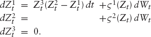
One popular example is Heston's model (2.1).

The interpretation of this observation is that if variance swaps are priced using Heston's model, which in turn is calibrated every day to market data, then the speed of mean reversion, Z³, must theoretically be kept constant. Using entropy swaps, it can also be shown [54], that the product of “vol of vol” and “correlation” in Heston's model must in theory be kept constant.

Also note that this example covers by a simple coordinate transformation the Nelson-Siegel interpolation function for interest rates, G(z; x) = z₁ + (z₂ + z₃)e^−z4x. More generally, assume that G is a polynomial exponential, that is, that G is of the form

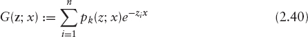
for polynomials and n ≤ m. Using (2.39), it is straightforward to show that the “speeds of mean reversion” Z¹, …, Zⁿ for any consistent parameter process must be constant. A similar result holds for functions of the form in which case the parameters z₁, …, z_n must not only be constant, but also need to come in pairs in which one is twice the value of the other parameter. The observation that speeds of mean reversion must generally be constant for interest rate models was first shown by Björk/Christensen [55] and further investigated by Filipovic [52].

Another example of functionals of the class (2.40) is given by, G(z; x) = z₁ + (z₂ + z₃)e^−z₄x + z4e^−z₅x. Following Buehler [49], we use the following reparametrization, which makes it easier to ensure that the function remains positive:

EXAMPLE 6 The “double linearly mean-reverting” variance curve functional is defined for positive constants κ and c as

with a well-defined limit for κ = c. A consistent parameter process follows an SDE of the form

For the case in which Z¹, …, Z³ are square roots of affine functions, such a process fits in the affine framework of Duffie et al. [56]. The curve (2.41) has proven to be a good interpolation for actual market data; an example is given in figure 2.20. Also recall that we have shown in section 2.1.5 that in the case and ζ² = ζ³ = 0, a semi-closed form for European option prices can be derived. We will discuss a model based on (2.41) below.

While the linearly mean-reverting models admit a range of possible parameter processes, this is not generally true. Here is an example of a curve that admits only one parameter process:

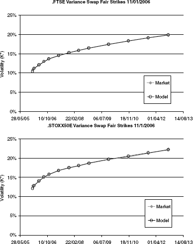
FIGURE 2.20 Fit of the double mean-reverting functional (2.41) to FTSE and STOXX50E market data.

EXAMPLE 7 For the “exponential linearly mean-reverting” variance curve functional

any parameter process Z is constant in Z², Z³ and Z⁴. The parameter Z¹ follows an Ornstein-Uhlenbeck process

that is, G is driven only by Scott's exponential OU model.

It is also interesting to see whether a functional admits a parameter process at all. To this end, note that sometimes functions like are used to interpolate the term structure of implied volatility. Applied to variance swap curves, though, it can be seen easily that such an interpolation of the variance swap volatility, that is, using G(z, x):= xg²(z; x), does not admit a consistent parameter process. This observation means that at least in the case of flat skew, implied volatility cannot consistently be interpolated with such functions.

REMARK 2.3.3 The results here are of a theoretical nature. In practice, the speed of mean reversion of a Heston model must be calibrated to market data, and we cannot enforce a constant value over a long period of time without considerably weakening the fit of the model to the market. Moreover, it should be clear that a real trading desk faces many more inconsistencies arising from trading in the real world.

From this point of view, the results here regarding a constant mean reversion should be merely taken as advice to avoid strong movements of the parameter as a result of the daily recalibration of the model. Indeed, in our experience, imposing a penalty on movements of the speed of mean reversion during calibration leads to a much more stable daily recalibration of, for example, Heston's model.

A Double Mean-Reverting Model Following example 6, a convenient parametrization to drive the double linearly mean-reverting curve functional (2.41) is given by

and

The correlation structure of the involved Brownian motions is given in terms of the parameters ρ_ζ, ρ_θ, r_θ,ζ and ρ_m as

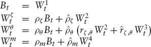
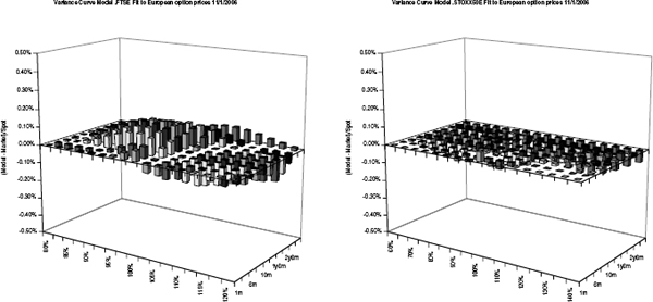
FIGURE 2.21 Calibration of the double mean-reverting model (2.42) to FTSE and STOXX50E market data. The variance swap fits are shown in figure 2.20.

(we used the notation The exponentials α and β are assumed to be from (0.5, 1) to ensure that (2.42) has a unique strong solution. To ensure that X is a true martingale, we assume that ρ_ζ, ρ_θ and ρ_m are negative.

The dynamics of this model are very intuitive: The short variance ζ is a mean-reverting process whose mean-reversion itself is stochastic. Such a behavior is often observed in real markets. The stochasticity of m has been introduced to fit the market slightly better, but in general and in the interest of parsimony, we usually set η = 0.

The calibration of the initial states ζ₀, θ₀, and m₀, along with the reversion speeds κ and c, can be done by fitting (2.41) to the observed variance swap market data. The remaining parameters ν, μ, α, β, ρ_ζ, and ρ_θ (r_ζ,θ is usually set to zero), on the other hand, require quite an expensive calibration via Monte Carlo. This is numerically far less robust than the calibration of, say, a Heston model. Indeed, to reduce the time spent during the calibration, we typically calibrate to only five maturities with three options per maturity. (While being theoretically attractive, such a model is necessary only if we want to price spread-type products such as forward-started options on variance). Figure 2.21 shows the calibration results for this model to STOXX50E and FTSE market data.

To assess the impact of the model choice, we also calibrated the model (2.11) with θ_t := m + (θ₀ − m)e^−ct and piecewise constant vol of vol and correlation to the same market data. It can be written as

and it also has the variance curve (2.41). The calibration results are shown in figure 2.22. Given the calibrated model, we can now price arbitrary options on variance. Figures 2.23 and 2.24 display the prices of calls on variance computed with the two calibrated models (all prices here are computed using Monte Carlo simulation with control variates on the variance swaps).

FIGURE 2.22 Calibration of the extended time-dependent Heston model (2.43) to FTSE and STOXX50E market data. The variance swap fits are shown in figure 2.20.

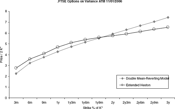
FIGURE 2.23 Prices of ATM calls on realized variances with the calibrated double mean-reverting and the calibrated extended Heston model (2.43).

2.3.3 Fitting to the Market

The previous sections discussed how we can model consistently the idea of “interpolating the variance swaps”: We assumed that if we find a suitable function that interpolates well the variance swaps at any time t, then we can derive no-arbitrage conditions on the dynamics of the parameters of this function. This approach is in spirit the idea of Björk/Christensen [55], who first introduced this concept of “consistency” for interest rates. However, by far more popular interest rate models are those that serve only two purposes: a perfect fit to the interpolated discount bonds, regardless of the interpolation method used, and a parsimonious specification of the volatility structure of the model. The best known models of this class are the one- and two-factor extended Vasicek or Hull-White models; see chapter 3.

FIGURE 2.24 Prices of 1y calls on realized variances with the calibrated double mean-reverting and the calibrated extended Heston model (2.43).

We will now discuss similar approaches for variance curves and thereby forgo the consistency approach. The aim is now to fit the market and to be able to describe the volatility structure of variance in a parsimonious way. We assume that we observe a sufficiently smooth variance swap market curve U₀ = (U₀(x))_x≥0 with forward non-negative forward variance curve u₀(x):= ∂_xU₀(x). Recall the fixed time-to-maturity quantities v_t(T) := u_t(T − t) and V_t(T) := U_t(T − t).

EXAMPLE 8 Dupire [57] proposed a “fitting stochastic volatility” model based on an exponential representation of the forward variance curve, that is,

where ν is a deterministic volatility function.

Indeed, this approach can easily be generalized. To this end, assume that we are given a variance swap curve model (G, Z). Then,

can be seen to be a variance curve model that reprices the variance swap market (i.e., u₀ ≡ u₀). A model very similar to Dupire's is therefore given by using Scott's exponential OU model,

where dw_t = −κw_t dt + ν dW_t is an Ornstein-Uhlenbeck process. We call this model “fitted log-normal.” It can be extended to a sum of correlated Ornstein-Uhlenbeck processes, as proposed by Bergomi [48]. However, following Jourdain [25], care should be taken with (2.44) to ensure that the associated stock price process is a true martingale (the local martingale property is ensured if the original model yields a local martingale for the stock price).

REMARK 2.3.4 Sin [58] makes the following observation: a local martingale

with nonexplosive short variance ζ is a true martingale if, and only if, the process ζ does not explode under the measure associated to the numeraire X.²²

Using this result we can show that (2.44) applied to Heston's model will retain the martingale property of the associated stock price as long the correlation ρ is not positive.

The drawback of the “fitted log-normal” model is that it is to our knowledge not possible to efficiently compute European option prices. That implies that we have to revert to expensive numerical methods if the model is to be calibrated to European prices. A model that does not have this drawback can be constructed from example (2.43) given earlier: we have discussed that European prices for

can be computed relatively efficiently using Fourier transforms provided θ is nonnegative. Since

it is easy to see that if we set θ_t := κu₀(t) + ∂_xu₀(x), then we fit the market: The non-negativity condition on θ essentially implies that u₀ must have the form u₀(x) = e^−κxf(x) for some increasing function f. As long as this condition is satisfied, we obtain a “fitted Heston model” that reprices the initial variance curve, which has a parsimonious parameter structure and which allows the calibration of these “volatility parameters” κ, ν and ρ via European options. Additionally, the volatility parameters can be made piecewise time dependent; cf. (2.12) and the discussion thereafter.²³

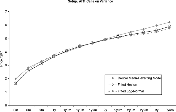
FIGURE 2.25 We have adjusted the parameters for the fitted Heston and fitted log-normal model by hand to roughly match ATM calls on variance between 1y and 2y of the double mean-reverting model. The graph shows the quality of the match and the impact on the short and long end of the ATM curve.

Model Dependency If we use a specific model to price and hedge an exotic payoff, we are subject to model risk. Hence, it is important to assess the impact of the choice of a model. To this end, we present here a few results on the comparison between the fitted Heston model, the fitted log-normal model and the double mean-reverting model (2.42). To be able to compare the models, we interpolate the variance swaps using the variance swap curve function (2.41). Next, we price a 100% ATM call on variance using the double mean-reverting model using the parameters calibrated in the examples before. Then, we adjust the parameters ν and κ in the fitted Heston and fitted log-normal model such that they both have very similar option prices for the 1y to 2y 100% ATM calls (the correlation parameters do not have a big impact on pricing of options on variance).

Having matched the models in this way, we can now compare the impact of the choice of a model first by comparing ATM calls with different maturities and second by comparing the prices of out-of-the-money calls. This is shown in figures 2.25 and 2.26. It is remarkable how similar prices the two fitted models produce: once the fitted log-normal and the fitted Heston agree for the ATM option, they produce very similar OTM option prices. Because of this very similar fit, the two models also produce very similar “VarSwapVegas”; hence, both price and hedge of a European option on realized variance are relatively robust with respect to model choice once the ATM calls are matched.

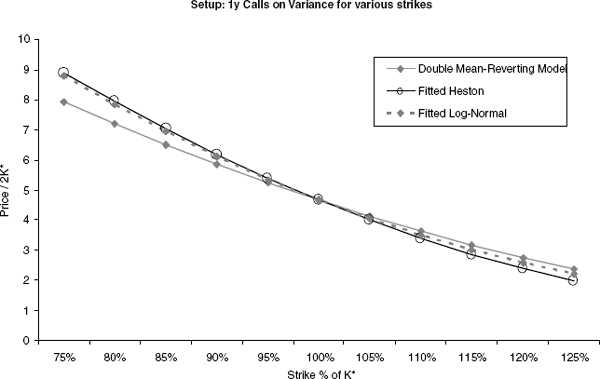
FIGURE 2.26 This graph shows the prices of 1y calls for the three models shown in figure 2.25.