
CHAPTER 9
Numerical Solution of Multifactor Pricing Problems Using Lagrange-Galerkin with Duality Methods
9.1 INTRODUCTION
Many financial derivative products are conveniently modeled in terms of one or more factors, or stochastic spatial variables, and time. Based on the contingent claims analysis developed by Black and Scholes [72] and Merton [73], a partial differential equation (PDE) for the fair price of these derivatives can be obtained. Valuation PDEs for financial derivatives are usually parabolic and of second order. In the more general case, partial differential inequalities (PDIs) arise. The inequality comes when the option has some embedded early-exercise features and the price of the contingent claim must satisfy some inequality constraints in order to avoid arbitrage opportunities. In other words, if the price were to violate those constraints, the option would be exercised, since both the buyer and the seller of an option will try to maximize the value of their rights under the contract. Early-exercise features appear, for example, in American options and in the conversion, call, and put provisions of convertible bonds. These are so-called free boundary problems because there are (a priori) unknown boundaries separating the regions where inequalities are strict from those where they are saturated.
It is almost always impossible to find an explicit solution to a free boundary problem: we need numerical techniques. The extra complication in those problems comes from the fact that we do not know where the free boundary is; it is an extra unknown that we need to find as part of the solution procedure. The most common method of handling the early exercise condition is simply to advance the discrete solution over a time step, ignoring the restriction, and then to make a projection on the set of constraints (see, for example, Clewlow and Strickland [139]). This is very easy to implement but has the disadvantage that the solution is in an inconsistent state at the beginning of each time step (see Wilmott, Dewynne, and Howison [140]).
Rigorous methods to deal with free boundaries transform the original problem into a new one having a fixed domain from which the free boundary can be found a posteriori. The problem may be formulated in two ways: The first is as a linear complementary problem (a strong formulation), usually combined with finite difference methods; the second is as a variational inequality (a weak formulation), usually related to finite element methods. The latter has some advantages. First, variational inequalities are an excellent framework to deal with issues such as existence and uniqueness of the solution. Second, they are appropriate to analyze the error incurred in the numerical methods (numerical analysis). Finally, writing a weak formulation is a necessary step in using finite element methods for numerical solution.
In this chapter, we present a framework for solving multifactor option-pricing problems with early-exercise features. We first introduce a duality (or Langrange multiplier) method to deal with inequality constraints in the solution or its derivatives. Then the method of characteristics and finite elements is proposed for time and space discretization, respectively. The combination of these numerical methods has been applied to finance by Bermúdez and Nogueiras [107] and Vázquez [141].
There are three main issues when using PDE methods in contingent claim valuation: (1) how to account for early-exercise features; (2) how to discretize the model; and (3) how to deal with the convection-dominance problem. The main goal, of course, is to achieve the best trade-off between speed and accuracy according to the circumstances of our valuation problem.1
In order to deal with free boundary problems, we first reformulate them in a mixed form by means of a Lagrange multiplier. Then we propose an iterative algorithm in which the solution of the nonlinear problem, that is, the problem with constraints, is approximated by a sequence of solutions of linear (unconstrained) problems. This algorithm is a particular application of the one introduced by Bermúdez and Moreno [142] and has been used extensively in other fields. The algorithm provides great generality in the sense that it allows for any type of constraint to be imposed on the value function or its derivatives, which may depend on the spatial variables and time. It can be applied to either the weak or the strong problem; hence, it can be combined with either finite difference or finite element discretization. Moreover, since the solution of the nonlinear problem is approximated by a sequence of solutions of linear problems, any existing code for discretizing partial differential equations could be easily extended.
Sometimes in finance the effect of the volatility term is smaller than the effect of the drift term, giving rise to the so-called convection-dominated problems. Furthermore, the diffusive term may become degenerate in the following senses: We may distinguish between weak degeneration, as in Black-Scholes where the diffusion vanishes for zero spot, or strong degeneration of ultraparabolic type, as in Asian options in which there is no diffusion in one direction. In such situations second-order centered space-discretization schemes may lead to spurious oscillations. In the tree framework this is equivalent to saying that the local drift is so large relative to the diffusion that branching into the usual binomial or trinomial tree will lead to negative probabilities. Hull and White [143] have solved this with their alternative branching technique. In a PDE approach, one has to resort to first-order, one-sided space differencing or to the more recent Eulerian and characteristics techniques, such as the ones described in Ewing and Wang [144]. The method of characteristics for time discretization is a possible approach to deal with convection-dominated problems. Its main advantages are:
- It is unconditionally stable even when applied to the transport equation (no diffusion). Hence, it copes well with degenerate diffusions.
- It yields discrete symmetrical linear systems, whose numerical solution is faster than nonsymmetrical ones.
The modified method of characteristics or semi-Lagrangian method was introduced in the 1990s by Pironneau [145] and Douglas and Russell [146]. It has been applied to convection-diffusion equations combined with space discretization using both finite differences (see [146]) and finite elements (see [147], [148], [149]). When combined with finite elements it is referred to as characteristics finite elements, or the Lagrange-Galerkin method. The classical method of characteristics is only first order accurate. However, higher order characteristic finite element methods have been proposed by Boukir et al. [150] and Rui and Tabata [151]. Bermúdez, Nogueiras, and Vázquez [152, 197] extended the method in Rui and Tabata and applied it to the valuation of American-Asian options. We describe the classical Lagrange-Galerkin method as well as the second-order scheme proposed in [152, 197].
While most papers and books on financial derivatives employ finite differences (FDs) for the numerical solution (see, for instance, Wilmott, Dewynne, and Howison [140]), the use of finite elements (FEs) has several advantages (see Ciarlet and Lions [153]):
- It can be used with domains of arbitrary geometries and arbitrary boundary conditions.
- It allows unstructured meshes, which can be convenient for making refinements in particular regions of the domain, such as around free boundaries or near barriers.
- It has a solid mathematical foundation. There is a well-developed theory about apriori and a posteriori error estimates, which allows a rigorous analysis and is a necessary tool for adaptive algorithms.
- It is well suited for modern computer architectures, particularly parallel processing.
This chapter is organized as follows: In section 9.2, we introduce the general modeling framework. In section 9.3, we describe the duality method to reduce the nonlinear problem to a sequence of linear problems. Section 9.4 describes the classical first-order Lagrange-Galerkin method, which can be used to solve the linear problem numerically. Section 9.5 introduces higher-order Lagrange-Galerkin schemes, and section 9.6 applies the classical Lagrange-Galerkin method to the valuation of convertible bonds.
9.2 THE MODELING FRAMEWORK: A GENERAL D-FACTOR MODEL
The fair price of many financial derivatives can be obtained by solving final-value problems for parabolic partial differential equations, eventually involving inequality constraints. These constraints could affect the option value, like in American-and Bermudan-style options or in convertible bonds, or may be imposed on the value of the spatial derivative of the solution, if we intend, for instance, to price a barrier option subject to a cap on the delta. Those are the so-called free boundary problems and are an example of nonlinear problems. Recall that free boundary problems may be mathematically formulated as linear complementary problems (strong formulation) or as variational inequalities (weak formulation). The terminology weak–strong refers to the regularity of the solution. Each solution of the strong formulation is a solution of the weak problem. Conversely, if a solution of the weak problem is smooth enough, then it is a solution of the original problem in the classical sense. Existence and uniqueness of a strong solution require the final and boundary conditions to be sufficiently smooth (payoff functions are generally not even differentiable). These constraints can be weakened when we use a weak formulation of the problem; the difficulties do not disappear, but solutions are sought in more general functional spaces (weighted Sobolev spaces).
In this section, we introduce a general d-factor pricing framework. First, we set the final-value linear problem in the absence of constraints. Then we formulate the nonlinear problem, both in strong and weak form. In order to use an iterative algorithm to deal with the free boundaries, we will need to reformulate the problem in a mixed form by means of a Lagrange multiplier. We will distinguish between the primal formulation, which involves only the unknown option price, and the mixed formulation, which involves the Lagrange multiplier as an extra unknown.
9.2.1 Strong Formulation of the Linear Problem: Partial Differential Equations
Let the value of a contingent claim φ be a function of time t and d spatial variables x = (x1, …, xd). Very often, the value φ of the contingent claim can be found as the solution of a parabolic partial differential equation of the following form:

where Ω is the spatial domain and Aij, Bi, A0 and f are given measurable functions of (x, t). Typically, xj represents quantities such as the value of an underlying asset or a stochastic interest rate. Therefore, they run either in the interval [0, ∞) or in the whole real line ![]() We also have to include the final condition, the payoff of the contract, which depends on the specific derivative product. In general, we will write
We also have to include the final condition, the payoff of the contract, which depends on the specific derivative product. In general, we will write
In order to obtain a weak formulation, we need to rewrite the equation in divergence form

where the new coefficients aij, bi, a0 are given by
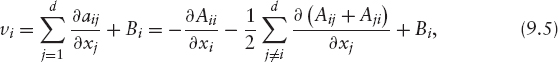
Notice that we have imposed symmetry to the matrix A = (aij). Equation (9.3) is simply a d-dimensional linear convection-diffusion-reaction equation, with diffusion matrix A = (aij), velocity vector v = (v1, v2, …, vd) (convection), and reaction coefficient a0.
It will be useful, for the following sections, to formulate the model using the material or total derivative of φ with respect to time t and the velocity field v, namely,

With this notation, equation (9.3) becomes

Denoting the differential operator by
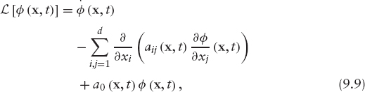
the pricing problem (9.1)–(9.2) may be written as
PROBLEM 1 Linear Problem (Strong Formulation)
Find ![]() such that
such that

9.2.2 Truncation of the Domain and Boundary Conditions
Very often, the pricing problem is a pure Cauchy problem; that is, only an initial condition is needed to guarantee existence and uniqueness of solution. However, numerical discretization, by using either finite difference, finite elements, or finite volume methods, makes it necessary to cut the domain at finite distance and to introduce “artificial” boundary conditions. Those are generally obtained by financial arguments, but also by pure mathematical reasoning, and have to be included in the weak formulation. This process, called localization, often arises in numerical finance, and introduces a model error that has been studied, for instance, by Kangro and Nicolaides [154] and by Barles et al. [162].
Let us still call Ω the bounded domain, and Γ its boundary. We denote ΓD (respectively ΓR) the subset of Γ where Dirichlet (respectively Robin) boundary conditions are imposed. Specifically,
where
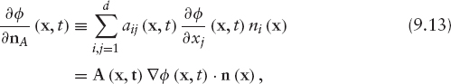
and n = (n1, …, nd) denotes a unit outward normal vector to Γ. In equations (9.11) and (9.12), functions α, g, and l are data.
In general, ![]() is a nonempty set in which no boundary conditions are needed because the natural condition for the weak formulation is identically satisfied. Specifically, Γ0 is the set where tA(x, t) n (x) = 0 and, therefore,
is a nonempty set in which no boundary conditions are needed because the natural condition for the weak formulation is identically satisfied. Specifically, Γ0 is the set where tA(x, t) n (x) = 0 and, therefore, ![]() (x, t) = 0 for any function φ.
(x, t) = 0 for any function φ.
The discussion on boundary conditions, sometimes ignored in financial literature, is often a complicated task and depends on the particular financial product.
REMARK 9.2.1 In a d-factor model the computational or “localized” domain Ω is frequently a rectangle [a1, b1] × [a2, b2] × … [ad, bd]. In such a case, the boundary Γ may be decomposed as:

where Γi+ (respectively Γi−) is the part of the boundary characterized by the unit outward normal vector
![]()
(respectively (0, …,−1(i), …,0)).
9.2.3 Strong Formulation of the Nonlinear Problem: Partial Differential Inequalities
Early-exercise features, in American options or convertible bonds, for instance, may be included in the model by means of unilateral constraints applied to φ. Hence, partial differential inequalities, rather than partial differential equations, have to be considered.
If φ (x, t) is the value of an American-or Bermudan-style option, extra constraints need to be added to Problem 1 in order to avoid arbitrage opportunities. Specifically, if the holder of the option has the right to exercise at time t and to receive an exercise value R1(x, t), then we need
In this case, φ (x, t) satisfies equation (9.10a) only if
![]()
If
![]()
then
Similarly, if the option may be exercised by the issuer2 at time t for an exercise value R2(x, t), we need
In that case φ (x, t) solves equation (9.10a) only if
![]()
If
![]()
We refer to (9.16) and (9.18) as partial differential inequalities (PDIs), and we call (9.15) and (9.17) unilateral conditions, restrictions or constraints.
The general nonlinear problem will be:
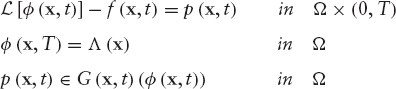
PROBLEM 2 Nonlinear Problem (Strong Primal Formulation)
Find ![]() , satisfying boundary conditions (9.11) and (9.12), such that
, satisfying boundary conditions (9.11) and (9.12), such that

The above is a so-called primal formulation, because it involves only the unknown φ. It is also called linear complementary problem. Problem (9.19) can be rewritten by introducing a Lagrange multiplier, leading to a so-called mixed formulation. Specifically, (9.19) is equivalent to:
PROBLEM 3 Nonlinear Problem (Strong Mixed Formulation)
Find functions ![]() satisfying boundary conditions (9.11) and (9.12) such that
satisfying boundary conditions (9.11) and (9.12) such that
and furthermore
with
Function p is a Lagrange multiplier, which adds or subtracts value in order to ensure that constraints in the solution are being met. Certainly, in the region where p = 0, the equality in (9.10a) holds. The surfaces separating the regions where p < 0, p = 0 and p > 0 are the so-called free boundaries.
Let us introduce the following family (indexed by x, t) of set- (or multi-) valued graphs defined by

It is straightforward to show that inequalities (9.21)–(9.24) are equivalent to the relation
Hence, Problem 3 may be rewritten as
PROBLEM 4 Nonlinear Problem (Strong Mixed Formulation)
Find φ (t) ∈ V satisfying boundary conditions (9.11) and (9.12) and p (t) ∈ M such that
where ν and M are suitable X-dependent function spaces for φ and p, respectively.
9.2.4 Weak Formulation of the Nonlinear Problem: Variational Inequalities
In order to discretize in space using the finite element method we have to rewrite the problem in a variational (or weak) form. We recall that variational inequalities are not only the starting point for the finite element discretization, but also constitute a powerful tool to deal with theoretical issues, such as existence and uniqueness of the solution as well as numerical analysis.
In order to write a weak formulation of the valuation problem we multiply equation (9.20a) by a test function ψ defined in Ω. Then we integrate in Ω to get
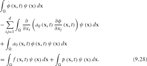
We use Green's formula to transform the second term on the left-hand side:

The boundary term in this equation is decomposed as (from 9.13):
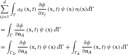
If we restrict the test functions to those vanishing on ΓD and replace ![]() on ΓR using boundary condition (9.11), we get
on ΓR using boundary condition (9.11), we get
Substitution into (9.29), and then of (9.29) into (9.28), yields

This is a so-called weak mixed formulation since both the primitive unknown φ and the Lagrange multiplier p are involved. In what follows, we will write another weak formulation that includes only the unknown φ.
Let us introduce the family of convex sets of functions defined, for each t in [0, T], by
where ν is a suitable space for φ.
Using (9.22), (9.23) and (9.24) it is straightforward to show that, for any ψ ∈ K(t) we have3
For each time t we replace the arbitrary test function ψ in (9.31) by κ − φ, where κ is in K(t) such that κ (x) = l(x, t) on ΓD. We get

Finally, we use (9.33) in this equality and obtain the following variational inequality of the first kind:
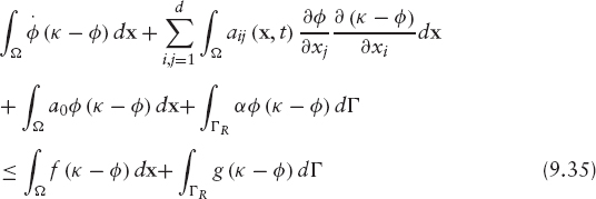
This is a weak primal formulation in the sense that now φ is the only unknown.
In order to write the problem in a more compact way, we introduce the following notations: Let a(t;·,·) be the family of bilinear symmetric forms
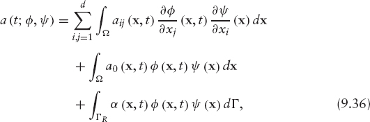
and L(t;·) be the family of linear forms:
Then the problem can be written in the two equivalent forms:
PROBLEM 5 Nonlinear Problem (Weak Primal Formulation)
Find φ (t) ∈ K(t) satisfying Dirichlet condition (9.12) and final condition (9.2) such that
PROBLEM 6 Nonlinear Problem (Weak Mixed Formulation)
Find φ (t) ∈ V and p(t) ∈ M satisfying unilateral conditions (9.21)–(9.24), Dirichlet boundary condition (9.12) and final condition (9.2) such that
where
and ν and M are suitable spaces for φ and p, respectively.
9.3 NUMERICAL SOLUTION OF PARTIAL DIFFERENTIAL INEQUALITIES (VARIATIONAL INEQUALITIES)
As mentioned before, the most common method of handling the early exercise condition is simply to advance the discrete solution over a time step ignoring the restriction and then to make a projection on the set of constraints. This is easy to implement, but a discrete form of the linear complementary problem or the variational inequality is not satisfied.
In the case of a single-factor American put, the algebraic linear complementary problems are commonly solved using a projected iteration method (PSOR) (see Wilmott [163], Vázquez [141]).
Clarke and Parrot [164] suggested a multigrid method to accelerate convergence of the basic relaxation method. They showed that the algorithm, when applied to the valuation of American options with stochastic volatility, gives optimal numerical complexity and the performance is much better than for the PSOR.
On the other hand, Forsyth and Vetzal [165] proposed an implicit penalty method for valuing American options and showed that when a variable time step is used, quadratic convergence is achieved. They derived sufficient conditions to guarantee monotonic convergence of the nonlinear penalty iteration and also to ensure that the solution of the penalty problem is an approximate solution to the discrete linear complementary problem. They compared the efficiency and the accuracy of the method with the commonly used technique of handling the American constraint explicitly in the tree methodologies. Convergence rates as the time step and the mesh size tend to zero for the standard CRR tree are compared with convergence rates for an implicit finite volume method with Crank-Nicolson time stepping and the penalty method for handling the American constraint. They found that the PDE method is asymptotically superior to the binomial lattice method.
Barone-Adesi et al. [97], Bermúdez and Nogueiras [107], and Bermúdez et al. [152, 197] used a Lagrange multiplier (or duality) method to solve variational inequalities arising in the valuation of convertible bonds and Amerasian options. This method has been introduced in [142] for solving elliptic variational inequalities of the second kind (see also Parés et al. [166] for further analysis). It has not been applied much in finance but has been used extensively in other fields such as computational mechanics. As mentioned in Section 9.1, the algorithm can be used for any type of constraint to be imposed on the value function or its derivatives, which may depend on the spatial variables and on time. It is based on the mixed formulation and could be applied to either the weak or the strong problem; hence it could be combined with either finite difference or finite element discretizations.
In this section, we describe this general methodology to solve the nonlinear problems introduced in the previous section. The solution of the nonlinear problem is approximated by a sequence of solutions of linear problems. In the next section, we describe the numerical solution of the linear problem using a discretization in time with characteristics and a discretization in space with finite elements. Finally, the Lagrange multiplier method is applied to the fully discretized problem.
9.3.1 A Duality (or Lagrange Multiplier) Method
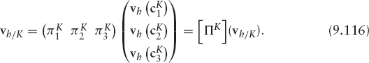
Recall that inequalities (9.21)–(9.24) establish a relationship between p and φ, which can be written in a more compact way as
where G(x, t) is the family (indicated by x, t) of set (or multi)-valued graphs introduced in (9.25).
Since G(x, t) is a multivalued function, equation (9.41) is not easy to implement. However, we have the following result (see Bermúdez and Moreno [142]):

FIGURE 9.1 Yosida approximation.
LEMMA 9.3.1 The following two statements are equivalent:
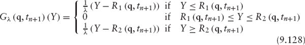
where Gλ(x, t) is the Yosida approximation of G(x, t) (see Figure 9.1) defined by

We notice that, unlike G,Gλ is a Lipschitz-continuous (univalued) function.
In view of this lemma and the previous discussion, relations (9.21)–(9.24) are equivalent to the following equality:
where λ is a positive real number.
We are now in a position to introduce the following iterative algorithm:
- At the beginning, the function p0 is given arbitrarily.
- At iteration m, an approximation of the Lagrange multiplier pm is known and we proceed as follows:
First, we work out a new approximation of φ(t), φm+1, by solving the linear problem in either weak- or strong-form
PROBLEM 7 Linearized Continuous Problem. Given pm ∈ ν, find φm+1 ∈ ν such that
Then, we update the Lagrange multiplier p by using equation (9.44). Precisely, pm+1 is defined as
where, in order to achieve convergence, λ has to be greater than some positive value which depends on coefficients aij, a0, and bi (see Bermúdez and Moreno [142] for details).
9.4 NUMERICAL SOLUTION OF PARTIAL DIFFERENTIAL EQUATIONS (VARIATIONAL EQUALITIES): CLASSICAL LAGRANGE-GALERKIN METHOD
In the previous section we introduced an iterative algorithm to approximate the solution of the nonlinear problem by a sequence of solutions of linear problems. Note that equations (9.45) and (9.46) are linear because, although they include the Lagrange multiplier, it is known from the previous iteration. What remains is to solve the linear problem by discretizing in time an space. We approximate equation (9.45) with a semi-discretization in time using the method of characteristics and a spatial discretization using finite elements. Recall that spatial discretizations using finite differences start with the strong formulation (9.46), whereas spatial discretization using finite elements are applied to the weak formulation (9.45). Time discretization using characteristics could be combined with both finite differences and finite elements.
9.4.1 Semi-Lagrangian Time Discretization: Method of Characteristics
The pricing equation is simply the convection-diffusion equation together with a reaction term producing an exponentially decay due to the discounting. Accurate modeling of the interaction between convective and diffusive processes is one of the most challenging tasks in the numerical approximation of partial differential equations; the choice of the numerical method depends on whether the problem is diffusion dominated or convection dominated. Sometimes, in finance, the diffusion is quite small relative to the convection, leading to a so-called convection-dominated problem. The numerical solution of convection-dominated problems is more complex than the solution of fully elliptic or parabolic equations. Problems arise due to the lack of natural dissipation embedded in parabolic partial differential equations, which helps make numerical schemes stable. Moreover, the solution of linear hyperbolic problems will only be as smooth as the initial solution; hence, the regularizing effect of the fully parabolic equation could be lost. In all such circumstances, standard finite element and finite difference approximations may present difficulties. A large literature has been built up on a variety of techniques for analyzing and overcoming those difficulties; books like Morton [167] are entirely devoted to the subject. A summary of numerical methods for time-dependent convection-dominated PDEs can be found in Ewing and Wang [144]. They provide a historical review of classical numerical methods and a survey of the recent developments on the Eulerian and characteristics Lagrangian methods. Eulerian methods use the standard temporal discretization, while the main distinguishing feature of characteristic methods is the use of characteristics to carry out the discretization in time.
The method of characteristics (or Lagrangian method) for time discretization is a possible approach for dealing with convection-dominated problems. It is part of the more general family of upwinding methods, which take into account the local flow direction. This approach is based on the discretization of the total (or material) derivative, introduced in (9.7), which is the time derivative along the characteristic lines. In other words, it is the derivative in time for a particle moving with velocity v (see (9.5)). In a Lagrangian coordinate system, one would only see the effect of diffusion, reaction, and the right-hand-side terms but not the effect of convection. Often, the solutions of the convection-diffusion PDEs change less rapidly along the characteristics than they do in the time direction. This explains why characteristic methods usually allow large time steps while still maintaining stability and accuracy.
When combined with finite elements, the method of characteristics is referred to as the characteristics finite element (or the Lagrange-Galerkin) method. Its main advantages are that it is unconditionally stable and that it yields discrete symmetrical linear systems.
The classical semi-Lagrangian or characteristics method is first-order accurate in time. Applications in finance have been developed by Vázquez [141], to solve the one-factor model arising in the valuation of American options; Pironneau and Hetch [168], to solve the two-factor model arising in the valuation of an American put on the maximum of two assets; and by Barone-Adesi et al. [97], Bermúdez and Nogueiras [107], and Bermúdez et al. [152, 197] in the valuation of convertible bonds and American-Asian options.
Characteristic Curves For given ![]() where
where ![]() the characteristic line through (x, t) associated with vector field v is the vector function Xe(x, t;·) solving the initial value problem
the characteristic line through (x, t) associated with vector field v is the vector function Xe(x, t;·) solving the initial value problem
It represents the trajectory described by the material point that occupies position x at time t and is driven by the velocity field v (see Figure 9.2). Under some regularity assumptions on v, the characteristic line-solving problem (9.49) is well defined in [0, T] and is unique for each initial condition (x, t).
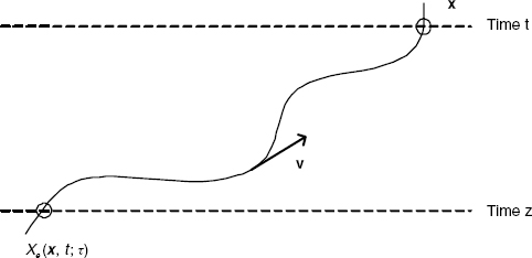
FIGURE 9.2 Characteristic line through (x, z) associated with vector field v.
From the definition of the characteristic curves and by using the chain rule, it follows that the material or total derivative, as defined in (9.7), satisfies

where φ′ denotes the partial derivative with respect to time and ![]() is the gradient.
is the gradient.
Approximation of the Material Derivative: Time Discretization In order to carry out a semidiscretization in time, we consider a partition of the time interval [0, T] into N time steps of size Δt = T/N that we will denote by tn = T − nΔt for n = 0, 1, …, N. Then, equation (9.50) suggests the following first-order approximation of φ at time tn+1
where we have used that Xe(x, tn+1; tn+1) = x.
The approximation (9.51) leads to the following implicit semidiscretized scheme for equation (9.45):
PROBLEM 8 Semi-Discretized Scheme
Given ![]() find
find ![]() for n = 0, …, N − 1, satisfying Dirichlet boundary condition
for n = 0, …, N − 1, satisfying Dirichlet boundary condition ![]() such that
such that

and
![]()
where φn+1(x) = φ(x, tn+1), pn+1(x) = p(x, tn+1), an+1(φ, ψ) = a(tn+1; φ, ψ) and Ln+1(ψ) = L(tn+1; ψ).
In most cases, the Cauchy problem (9.49) is not easy to solve analytically. However, the O(Δt) error of scheme (9.52) does not change if we replace Xe(x, tn+1; tn) by a first-order approximation given, for example, by an explicit Euler scheme
9.4.2 Space Discretization: Galerkin Finite Element Method
Galerkin methods are obtained by restricting both the solution and the test functions involved in the variational formulation to be in a finite dimensional space. In finite element methods, this space is made up of globally continuous functions that are polynomials in each element of a polygonal mesh of the domain Ω. In Galerkin methods, the solution and the test functions are looked for in the same finite dimension space. The solution of the PDE is built as a sum of all these local approximating functions. Usually, only the spatial variables are treated in this way, while time is discretized with FD or other methods. With two spatial variables, the domain is partitioned into triangles and/or quadrangles. Three-dimensional spatial domains allow partitions into tetrahedrons, hexahedrons, or prisms.
The distinction between FE and FD is relevant at the theoretical level, when dealing with the numerical analysis. Once the discrete scheme is written and one is left with algebraic transformations of values at the grid points, the distinction vanishes. On structured meshes, finite differences and finite elements plus specific numerical integration (using, for example, vertices) can be shown to be equivalent. The contrast should be seen more as variational methods versus finite differences rather than finite elements versus finite differences.
However, as mentioned in section 9.1, FE are more flexible than FD in incorporating boundary conditions and in that they allow unstructured meshes. As shown by Zvan et al. [110], unstructured meshing can be applied to a wide variety of financial models. The idea is that an accurate solution of the pricing PDE requires on many occasions a fine-mesh spacing in certain regions of the domain, usually where the gradient is steep, whereas in regions where the gradient is flat, a coarser mesh can be used. Some studies have indicated, for example, the need for small-mesh spacing near barriers (Figlewski and Gao [169], Zvan et al. [170]). Pooley [171] proves that the finite element method with standard unstructured meshing techniques can lead to significant efficiency gains over structured meshes with a comparable number of vertices for pricing barrier options. Pironneau and Hetch [168] present and test an adaptive algorithm for a problem with a free boundary that arises in finance for the pricing of American options, leading to satisfactory results.4
FE has some other computational practicalities compared to FD (see Winkler et al. [172]):
- FE is very suitable for modular programming.
- A solution for the entire domain is computed instead of isolated nodes as with the FD method.
- FE provides accurate “greeks” as a byproduct.
- FE can easily deal with irregular domains, whereas this is difficultly in FD.
Finite elements, which are a widely used technique in areas such as computational mechanics, have become quite popular in financial engineering. A recent text book is Topper [196].
Fully Discretized Lagrange-Galerkin Scheme In order to solve the Problem 8 numerically, a discretization must be done; in other words, the problem must be replaced by a new one with a finite number of degrees of freedom or unknowns.
As mentioned previously, Galerkin methods, replaces the space of functions ν by a finite dimensional space νh and defines a discrete counterpart of Problem 8 where the function φ is approximated by φh ∈ νh and the Lagrange multiplier p is approximated by ph ∈ νh. In finite elements, the space νh is made up of globally continuous functions that are polynomials in each element of a polygonal mesh of the domain Ω. Let us denote by Th a family of polygonal meshes of the domain Ω, where the parameter h tends to zero and represents the size of the mesh. We assume that the mesh contains Nhnodes and that any function in νh is uniquely defined by its values at the nodes. If ψ ∈ νh we call the values ψ(qi)j, i = 1, …, Nh the set of degrees of freedom. As in the continuous problem, we define
The discrete problem can be written as:
PROBLEM 9 Fully Discretized Scheme
Given ![]() find
find ![]() for n = 0, 1, …, N − 1 such that
for n = 0, 1, …, N − 1 such that

and
for all nodes q of the mesh Th, where Λh is the interpolated function of Λ in the space νh.
Let us define the bilinear form
and the linear form

Then Problem 9 above can be rewritten as:
PROBLEM 10 Given ![]() find
find ![]() satisfying Dirichlet boundary condition (9.55) such that
satisfying Dirichlet boundary condition (9.55) such that
Let us ignore for the moment Dirichlet boundary condition (9.55), in other words, let us assume that νh = ν0,h.
Let B = {φ1, φ2, …, φNh} be a basis of νh. Then the solution of (9.60) can be written (we omit indices for the sake of simplicity) in the form
so that the discrete problem (9.60) is equivalent to finding Nh numbers (ξ1, ξ2, …, ξNh) satisfying

Equivalently:
PROBLEM 11 Find (ξ1, ξ2, …, ξNh) ∈ ![]() such that
such that

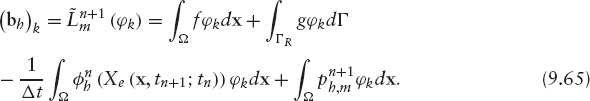
Since the matrix A is symmetric (see (9.4)), Ah is symmetric as well. If additionally Ah is positive definite, Cholesky's method can be used to solve the system (9.63). In the special case where coefficients aij, a0, and α do not depend on time, the linear system has a matrix independent of both time step and iteration; therefore, it needs to be computed and factorized only once. Also, in expression (9.65) the first two terms on the right hand side are independent of time (if f and g are) and iteration, whereas the third term must be computed at every time step, and the fourth at every time step and iteration. Consequently, in order to solve these systems it is convenient to use Cholesky or, more generally, direct Gauss-like methods, because, since the factorization step needs to be done only once, at each iteration just two triangular systems have to be solved.
In Problem 11 we have not taken into account Dirichlet boundary conditions. More precisely, we have included test functions φi in the basis of νh that do not satisfy the boundary condition ψi/ΓD = 0. Eliminating these functions of the basis is equivalent to eliminate the corresponding unknowns and equations (degrees of freedom). This process turns out to be unpleasant from the programming point of view. A simpler procedure is to replace the i-th equation (assuming the node i belongs to ΓD) by the equation
![]()
Actually the i-th equation is replaced by the “programming equivalent” obtained by substituting the diagonal term (Ah)ii by a large number, say H, and the right-hand side by Hl(qi). This process is called blocking of the degrees of freedom.
The problem arising now is how to choose the basis B = {φ1, φ2, …, φNh}. The elements of a suitable basis are functions that become zero in big regions of Ω so that many terms of the matrix Ah are zero; that is, Ah is a sparse matrix. We also need an efficient algorithm to work out the matrix of coefficients, Ah, and the right-hand-side vector bh, since the calculation of Ah and bh using formulas (9.64) and (9.65) is inefficient.
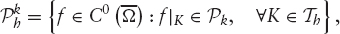
In the appendix, we consider Lagrange triangular finite elements in a d-dimensional domain Ω. We will show how to build the matrix of coefficients and the independent term in the particular case of Lagrange triangular finite elements of degree one in two space dimensions. This finite element space consists of continuous piecewise linear functions on a triangular mesh of the domain Ω. Specifically,
where C![]() denotes the space of continuous functions defined in
denotes the space of continuous functions defined in ![]() and P1 represents the space of polynomials of degree less than or equal to one in two variables. In this case the basis function φi takes value 1 at the vertex i of the mesh of the domain and is zero at all other vertices. We refer to Ciarlet [180] and Zienkiewicz et al. [181] as reference textbooks in the finite element method.
and P1 represents the space of polynomials of degree less than or equal to one in two variables. In this case the basis function φi takes value 1 at the vertex i of the mesh of the domain and is zero at all other vertices. We refer to Ciarlet [180] and Zienkiewicz et al. [181] as reference textbooks in the finite element method.
The Iterative Algorithm The algorithm we have introduced in section 9.3 to solve the continuous variational inequalities can now be written in summarized form for the fully discretized problem.

- At iteration m, we know

- We first compute
 as the solution of the linear problem
- Then we update the Lagrange multiplier using formula (9.48)

for all nodes q of the mesh Th where
By applying the results of convergence in Bermúdez-Moreno [142] we know that, for λ sufficiently large, the sequence ![]() converges to the solution
converges to the solution ![]() as m goes to infinity.
as m goes to infinity.
Figure 9.3 shows a flow chart of the complete algorithm: Lagrange-Galerkin combined with the iterative procedure.

FIGURE 9.3 Iterative method combined with Lagrange-Galerkin discretization.
9.4.3 Order of Classical Lagrange-Galerkin Method
There is a broad literature analyzing the classical first-order characteristic method combined with finite elements applied to convection diffusion equations. Suli [182] showed error estimates of the form O(hk + Δt) in l∞ (L2(Ω)) norm, where Δt denotes the time step, h the spatial step, and k the degree of the finite element space.5 Pironneau [145] stated error estimates of the form O(hk + Δt + hk+1/Δt) in l∞ (L2 (Ω)) norm under the assumption that the normal component of the velocity field vanishes on the boundary of the spatial domain and for an approximate discrete velocity field. In both cases, the constants depend on the norm of the solution. More recently, Bause and Knabner [183] proved convergence of order O(h2 + min(h, h2/Δt) + Δt) for linear finite elements and zero velocity on the boundary, where the constants on the error estimates depend only on the data.
9.5 HIGHER-ORDER LAGRANGE-GALERKIN METHODS
In order to obtain a better accuracy in space, it is necessary to use finite element spaces of higher order. In order to achieve a better accuracy in time, it is necessary to use higher-order characteristic methods. The latter consists of higher-order schemes for the discretization of the total derivative (9.7). There are two main approaches: multilevel schemes, which use a multistep formula to approximate the total derivative, and Crank-Nicolson schemes, which use a centered formula. Specifically, for fixed (x, t) = (x, tn+1) the following two second-order formulae could be used to approximate the material derivative:
![]()
The exact characteristic lines can be replaced by second-order approximations keeping still the O(Δt2) error. Possible schemes are:


Ewing and Russel [184] introduced multistep Lagrange-Galerkin methods for the convection-diffusion equation with constant coefficients. Boukir et al. ([150], [185]) also used multistep characteristics combined with either mixed finite elements or spectral methods to solve the incompressible Navier-Stokes. They proved the stability of the method and obtained error estimates.
Rui and Tabata [151] proposed a second-order Crank-Nicolson characteristic method for the convection-diffusion equation with constant coefficients and Dirichlet boundary conditions, with the exact characteristics approximated using a Runge-Kutta scheme. Bermúdez et al. [152, 197] extended their work to variable coefficients, possibly degenerate diffusion, nondivergence-free velocity field, non-zero reaction, and more general Dirichlet-Robin boundary conditions.
9.5.1 Crank-Nicolson Characteristics/Finite Elements
In section 9.3 we showed how the solution of the nonlinear problem could be written as the limit of solution of linear problems. In section 9.4 those linear problems were discretized using first order Lagrange-Galerkin schemes. In this section, we describe the second-order Lagrange-Galerkin method proposed by Bermúdez et al. [152, 197] for solving the general linear problem (9.10) together with boundary conditions (9.11) and (9.12). First, we write the weak formulation and then the semi-Lagrangian time discretization using both exact and approximate characteristics. Finally, we write the fully discretized problem and address some of the results in Bermúdez et al. [152, 197].
Weak Formulation We proceed to write a weak formulation of equation (9.3). Given that we will carry out a semi-discretization in time using characteristics, we first write equation (9.3) at point Xe(x, t; τ) and time τ giving (see (9.50)),
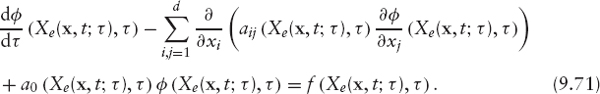
Equivalently, in vector notation

We will use the following notation:

In order to write a weak formulation, we need the following lemma.
LEMMA 9.5.1 Let ![]() be an invertible vector valued function. Let F =
be an invertible vector valued function. Let F = ![]() X and assume that detF
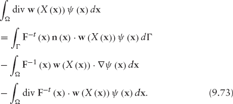
X and assume that detF ![]() Then for smooth vector field w and scalar field ψ, we have:
Then for smooth vector field w and scalar field ψ, we have:
Proof: See Bermúdez et al. [152, 197]
Note that equation (9.73) can be considered a Green's formula. Also, substitution of (9.74) into (9.73) yields
To write a weak formulation we multiply equation (9.72) by a test function ψ satisfying ψ = 0 on ΓD, integrate in Ω, and use the Green's formula (9.75) with X(x) = Xe(x, t; τ) and w = A![]() φ, obtaining
φ, obtaining

Now, using Robin condition (9.11), the boundary term in the above formulation can be rewritten as
Substitution of (9.77) into (9.76) yields

This is a weak formulation of equation (9.3). Note that if τ = t it reduces to the weak formulation in (9.31) with p = 0 (since we are solving the linear problem).
Second-Order Semidiscretized Scheme with Exact Characteristic Lines In order to carry out a semidiscretization in time, we consider a partition of the time interval [0, T] into N time steps of size Δt = T/N that we will denote by tn = T − nΔt for ![]()
We introduce the following notation:
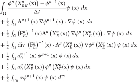
The method proposed in [152, 197] consists of fixing t = tn+1, n = 0, 1, …,N − 1 in the weak formulation (9.78) and applying a Crank-Nicholson scheme with respect

where we have used that Xe(x, tn+1; tn+1) = x and Fe(x, tn+1; tn+1) = I, I being the identity matrix.
Bermúdez et al. [152, 197] proved that the scheme (9.79) is of order O(Δt2) at point ![]()
Second-Order Semidiscretized Scheme with Approximate Characteristic Lines As mentioned before, in most cases the system of characteristics (9.49) cannot be solved exactly. Following Rui and Tabata [151], the exact characteristic lines, ![]() (x), could be replaced in (9.79) by a numerical approximation using an explicit method, like the first-order Euler scheme (9.53), or second-order Runge-Kutta scheme (9.69). As before, we will denote this approximations by
(x), could be replaced in (9.79) by a numerical approximation using an explicit method, like the first-order Euler scheme (9.53), or second-order Runge-Kutta scheme (9.69). As before, we will denote this approximations by ![]() (x) and
(x) and ![]() (x), respectively.
(x), respectively.
Thus, we are left with the following second-order approximation to (9.79) in the case the characteristic lines are not known explicitly:

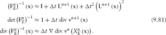
Note that, in order to preserve the O (Δt2) error bounds, it is necessary to use a second-order approximation of the characteristics lines in one term only. Besides, similarly to the exact characteristic case, det ![]() could be replaced by their O (Δt2) approximations below, avoiding the inversion of matrix
could be replaced by their O (Δt2) approximations below, avoiding the inversion of matrix ![]() Indeed, given
Indeed, given
![]()
it can be shown (see [152, 197]) that
Bermúdez et al. [152, 197] proved stability in l∞(L2) norm of scheme (9.80) under some hypothesis on the data and sufficiently small time step. Also, under further regularity assumptions on the data, they proved l∞(L2) error estimates of order O (Δt2) for the semidiscretized in time scheme.
Fully Discretized Lagrange-Galerkin Scheme In Bermúdez et al., [152, 197] a fully discretized Lagrange-Galerkin scheme is proposed for a wide class of finite element spaces. Let ![]() be a family of finite element spaces, where h denotes the space parameter and k is the “approximation order” in the following sense:
be a family of finite element spaces, where h denotes the space parameter and k is the “approximation order” in the following sense:
“There exists an interpolation operator ![]() satisfying
satisfying
![]()
for a positive constant K independent of h.”. 6.
Notice that the finite element space (9.66) falls into this family for k = 1. The fully discretized scheme reads as follows:
PROBLEM 12 Fully Discretized Second Order Scheme
Given ![]() such that
such that
where
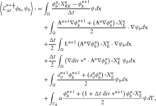
and
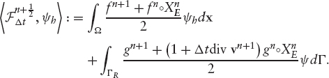
In Bermúdez et al. [152, 197] stability results for the fully discretized scheme (9.82) and error estimates of order O (Δt2) + O (hk) in l∞ (L2) norm are proved. These results are under the hypothesis that all inner products in the Galerkin formulation are calculated exactly. However, in practice numerical integration has to be used to approximate these integrals. Quadrature formulae have to be carefully chosen in order to preserve stability and the above order in the error estimates.
Specifically, in [152, 197] the following finite element spaces are considered
- For a family of rectangular meshes of parameter h, Th

where Qk is the space of polynomials of degree less than or equal to k in each variable separately.
- For a family of triangular meshes of parameter h, Th
where Pk is the space of polynomials of degree less than or equal to k.
They carried out some numerical tests in two space dimensions to illustrate the theoretical results regarding second-order Lagrange-Galerkin schemes combined with quadrature. It is well known that for the classical first-order-in-time Lagrange-Galerkin method, numerical integration may lead to conditional stability (see [184], [186], [187]). They did not find any sign of instability when using scheme (9.82) combined with either ![]() and the tensor product of the Simpson rule in each coordinate or
and the tensor product of the Simpson rule in each coordinate or ![]() with a seven-point quadrature formula. In both cases, an extra term of the form O(1/Δt) appears in the estimates of the error for fixed h. This agrees with evidence found for the first-order Lagrange-Galerkin scheme ([145], [187]).
with a seven-point quadrature formula. In both cases, an extra term of the form O(1/Δt) appears in the estimates of the error for fixed h. This agrees with evidence found for the first-order Lagrange-Galerkin scheme ([145], [187]).
They also carried out a comparison between the second-order Lagrange-Galerkin and the classical first-order scheme. Some of their results are shown in Figures 9.4 through 9.7. Example 1 in Figures (9.4) through (9.6) shows specific numerical solutions obtained with first- and second-order discretization in space. Example 2 in figure (9.7) shows the first- and second-order convergence in the time discretization.

FIGURE 9.4 Exact solution of the rotating Gaussian hill problem with T = 2 (Source: Nogueiras [198]).

FIGURE 9.5 Second-order characteristics with second-order ![]() FE. Numerical solution for the rotating Gaussian hill problem with T = 2. Mesh parameters are h = 0.015625 and Δt = 0.01. (Source: Nogueiras [98]).
FE. Numerical solution for the rotating Gaussian hill problem with T = 2. Mesh parameters are h = 0.015625 and Δt = 0.01. (Source: Nogueiras [98]).

FIGURE 9.6 Second-order characteristics with first-order ![]() FE. Numerical solution for the rotating Gaussian hill problem with T = 2. Mesh parameters are h = 0.015625 and Δt = 0.01. (Source: Nogueiras [98]).
FE. Numerical solution for the rotating Gaussian hill problem with T = 2. Mesh parameters are h = 0.015625 and Δt = 0.01. (Source: Nogueiras [98]).

FIGURE 9.7 Second order ![]() FE and different characteristics methods. l∞ (L2) norm of numerical error in log-log scale for a convection-(strong degenerated)-diffusion-reaction problem with variable coefficients.(Source: Nogueiras [98]).
FE and different characteristics methods. l∞ (L2) norm of numerical error in log-log scale for a convection-(strong degenerated)-diffusion-reaction problem with variable coefficients.(Source: Nogueiras [98]).
Overall, the second-order scheme outperforms the first-order scheme in terms of trade-off between the speed and the accuracy.
9.6 APPLICATION TO PRICING OF CONVERTIBLE BONDS
In this section, we apply the numerical methods described in this chapter to the valuation of convertible bonds. We consider the intensity-based framework for pricing convertible bonds described in section 4.4.
We study the convergence of the numerical method using the special case of a bond convertible only at expiry. Then we show prices for a real bond. Section 9.6.1 describes the numerical solution, and section 9.6.2 gives the numerical results.
9.6.1 Numerical Solution
The valuation of convertible bonds can be considered as a special case of the more general two-factor model presented in section 9.2. Moreover, the model in section 4.4.2 is a special case of the Problem 3 for the choices:
and
The Interest Rate Model We assume the interest rate follows the extended Vasicek model introduced in 3.1. This model combines tractability with the flexibility to calibrate to a prespecified initial term structure. We recall that the short-rate process under the EMM is
where θ(t) can be chosen so that model spot rates coincide with market spot rates.
9.6.2 Numerical Results
In this section, we show numerical results obtained when using classical Lagrange-Galerkin methods to price an actual CB, the Adidas-Salomon issue maturing on October 8, 2018. The evaluation date is December 16, 2005; hence, the time to maturity of the convertible expressed in years is
The bond has face value
and can be converted until September 20, 2018, at the rate (see Table 9.1)
TABLE 9.1 Conversion schedule for Adidas-Salomon convertible bond

TABLE 9.2 Call schedule for Adidas-Salomon convertible bond
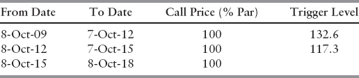
TABLE 9.3 Put schedule for Adidas-Salomon convertible bond
| Date | Put Price (% Par) |
| 8-Oct-09 | 100 |
| 8-Oct-12 | 100 |
| 8-Oct-15 | 100 |
The Adidas-Salomon issue is continuously soft-callable, that is, the stock price has to be above the trigger level before the call can be exercised; the call schedule is in table 9.2.
It is also puttable at par at three-year intervals, as shown in table 9.3.
The bond pays a 2.5% coupon annually on July 12.7
We assume a constant volatility for the underlying stock of σS = 23%, a continuous dividend yield d = 1.5868% and a repo rate q = 0.4%. We obtain ρ = −0.0188 for the correlation between the short rate and the equity, using the one-month EUROLIBOR as a proxy for the instantaneous rate (see figures 9.8 and 9.9).8
The extended Vasicek model (9.90) has been calibrated to market data as of December 16, 2005 (see section 3.3.1). The following values were obtained for the interest rate volatility parameters:

FIGURE 9.8 Adidas-Salomon daily stock price from January 1, 1998, to January 12, 2006.

FIGURE 9.9 One-month LIBOR daily rates from January 1, 1998, to January 12, 2006.
We use for the default specification λ = 0.0055, η = 1 and R = 40%. The instantaneous interest rate is r = 2.3804% and the stock price S = 157.54.
Convergence test In order to test the numerical method, we consider the special case of bond convertible only at expiry, for which we have an analytical solution (see section 4.4.4) and therefore we can compute the errors.
We set
given that there is no early-exercise embedded options.
Domain bounds are set to be Ωr = [0, 1.5] and ΩS = [9, 2077]. ΩS corresponds to roughly a 99.9% confidence interval on ST. We give L2 errors over both the entire domain Ω and also over a narrower region of interest ![]() where
where ![]() and
and ![]() is roughly a 99% confidence interval on ST.
is roughly a 99% confidence interval on ST. ![]() reflects a range of values of r and S likely to be observed in practice and so the error on
reflects a range of values of r and S likely to be observed in practice and so the error on ![]() is likely to be more representative.
is likely to be more representative.
We present results obtained for successive grid refinements for the relative error in L2. Mesh 1 is the coarsest with just 15 space steps in the interest rate dimension, 40 in the stock dimension, and 120 time steps up to time T = 3.5. Each successive mesh doubles both the number of space steps in each dimension and the number of time steps so that the finest mesh, mesh 4, has 120 interest rate steps, 320 equity steps, and 280 times steps. We use as a benchmarking measure the total relative error define as

where
and
errort = exact solutiont − numerical solutiont.
TABLE 9.4 Error and convergence

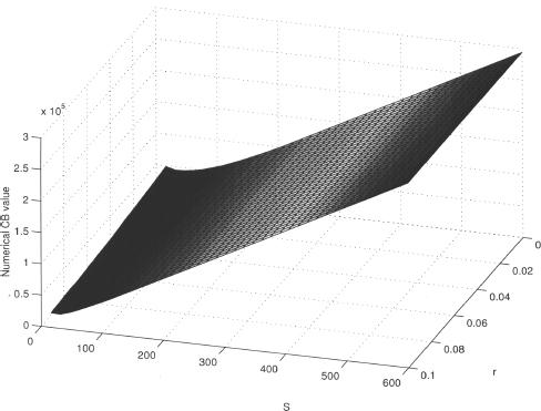
FIGURE 9.10 Numerical solution at evaluation date.

FIGURE 9.11 Lagrange multiplier at evaluation date.
The analytical formulae for the “exact solution” was given in (4.27); the value of the “exact solution” for the current level of the interest rate and the stock price is 79674.4525.
The numerical results are presented in table 9.4. On the boundaries we use the analytical solution. In each case two of the boundaries are Dirichlet and two are Neumann. “Error TD” is the error on the entire domain Ω; “Error RI” is the error on the region of interest, ![]() . “Factor” is the progressive error reduction factor in moving to a finer mesh level from the preceding mesh level.
. “Factor” is the progressive error reduction factor in moving to a finer mesh level from the preceding mesh level.
As mentioned in section 9.4.3, the classical Lagrange-Galerkin method is unconditionally stable and has convergence order of ![]() under suitable conditions for the coefficients of the equation. Although our models do not satisfy the required assumptions, the same error estimate has been obtained empirically. In table 9.4 it can be seen that the ratio between two consecutive errors tends to 2, which is consistent with the order of convergence given above.
under suitable conditions for the coefficients of the equation. Although our models do not satisfy the required assumptions, the same error estimate has been obtained empirically. In table 9.4 it can be seen that the ratio between two consecutive errors tends to 2, which is consistent with the order of convergence given above.
Pricing of a real CB Finally, we show the numerical solution for the Adidas-Salomon issue maturing on October 8, 2018, as of December 16, 2005. Figure 9.10 shows the CB prices, and figure 9.11 the Lagrange multiplier. Results were computed with mesh 4.
9.7 APPENDIX: LAGRANGE TRIANGULAR FINITE ELEMENTS
9.7.1 Lagrange Triangular Finite Elements in 
The domain ![]() is decomposed into simplices of dimension d (triangles if d = 2, tetrahedra if d = 3, etc.) and the space νh is the space of continuous functions in
is decomposed into simplices of dimension d (triangles if d = 2, tetrahedra if d = 3, etc.) and the space νh is the space of continuous functions in ![]() that are polynomials of degree smaller than or equal to k over any single simplex.
that are polynomials of degree smaller than or equal to k over any single simplex.
A set of d + 1 points {c1, …, cd+1 not lying on the same hyperplane is considered, is, such that the matrix

has a nonzero determinant.
The convex hull of these d + 1 points
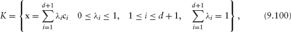
is called a d-dimensional simplex in ![]()
If x ∈ K the corresponding λi(x) = λi are known as barycentric coordinates of x. Notice that
![]()
and that λi is an affine function (polynomial of degree one) in the variables xj.
The subsets of K obtained when the following conditions are imposed
![]()
are called d − r dimensional faces of K.9
The barycenter of K is the point that has all the barycentric coordinates equal,
![]()
Let K be a d-simplex and k a positive integer; the subset of points of K
is called a lattice of order k in K. Note that the lattice of order k in K has ![]() elements.
elements.
Let Pk be the space of polynomials of degree equal to or less than k. Since a homogeneous polynomial of d variables and degree j has ![]() terms, the dimension of Pk is
terms, the dimension of Pk is
It can be shown that any polynomial of degree k is uniquely determined by its values at the ![]() points of the lattice of order k in K.
points of the lattice of order k in K.
With the triple ![]() we will build spaces of approximation νh.
we will build spaces of approximation νh.
Let Th be a partition of ![]() into simplices such that every face of a simplex Ki of Th is either:
into simplices such that every face of a simplex Ki of Th is either:
- A subset of ΓD,
- A subset of ΓR,
or
- A face of another simplex Kj of Th; in such a case Ki and Kj are said to be adjacent.
The diameter of K is denoted by hK and h = max {hK, K ∈ Th}. For k ≥ 1 the following functional spaces are built associated to Th
Clearly,

This inclusion simply states that any function of ![]() is a polynomial of degree equal to or less than k over each individual element. Conversely, what is the necessary and sufficient condition for an element of
is a polynomial of degree equal to or less than k over each individual element. Conversely, what is the necessary and sufficient condition for an element of ![]() to be in
to be in ![]() , that is, for the polynomial pieces to stick with continuity? The above will hold if and only if for every pair of adjacent elements Ki and Kj, the pieces defined on them agree on the points
, that is, for the polynomial pieces to stick with continuity? The above will hold if and only if for every pair of adjacent elements Ki and Kj, the pieces defined on them agree on the points
Therefore, any function in ![]() is uniquely determined by its values at the points of the set
is uniquely determined by its values at the points of the set
From now on, Th will be called a triangulation of Ω (even if the dimension d is different from 2) and the elements of ![]() nodes of the triangulation. Notice that there can be nodes that are not vertices.
nodes of the triangulation. Notice that there can be nodes that are not vertices.
The dimension of space ![]() is the same as the number of nodes. Also, it is possible to define a basis of
is the same as the number of nodes. Also, it is possible to define a basis of ![]() such that its elements are functions with support reduced to a few elements of Th. Let Nh be the number of nodes that we will assume to be numbered.
such that its elements are functions with support reduced to a few elements of Th. Let Nh be the number of nodes that we will assume to be numbered.
Node qi contributes to the basis with function ![]() uniquely determined by
uniquely determined by
9.7.2 Coefficients Matrix and Independent Term in Two Dimensions
We consider the problem in two dimensions (d = 2). Let us see how to organize the calculations to build Ah and bh in (9.64) and (9.65), respectively, if we choose the space of Lagrange triangular finite elements of degree one,
First, we consider the calculations ignoring the boundary condition on ΓD.
Let ![]() be the set of nodes of the triangulation Th that we will assume to be numbered
be the set of nodes of the triangulation Th that we will assume to be numbered
Notice that the dimension of ![]() equals Nh. Any node qj defines an element in the basis
equals Nh. Any node qj defines an element in the basis ![]() such that
such that
Then the solution φh can be written as
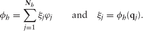
Therefore, the column vector (φh(q1), …,φh(qNh))t is the solution of the linear system (9.63). The calculation of Ah and bh using formulas (9.64) and (9.65) respectively, is inefficient because the same integrals are calculated several times over the same triangles. The method described below, which is the one used in practice, is based on the concepts of elementary matrix and assembling. The idea is that we will compute the contribution to the matrix and right-hand side vector over each individual element of the triangulation and then we will assemble them together in a systematic way to build the global approximation of the solution.
Let us recall that the discretized problem in two dimensions (ignoring Dirichlet boundary conditions) can be written as follows:
PROBLEM 13 Find ![]() such that
such that

where

Let us consider the first term of the left-hand-side of this equality. We have that
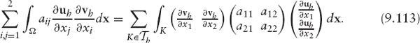
Let ![]() be the vertices of the triangle K and m1K, m2K, m3K the corresponding indices in the numbering of Th, that is assume
be the vertices of the triangle K and m1K, m2K, m3K the corresponding indices in the numbering of Th, that is assume
Let ![]() then
then ![]() where
where ![]() is the only polynomial of degree equal to or less than one, such that
is the only polynomial of degree equal to or less than one, such that
Equivalently,
Therefore,

Substitution of (9.117) into (9.113) yields
A similar process for the other terms leads to the following formulation of Problem 13:
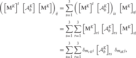
We introduce the Boolean matrix

such that, for any vector v of Nh components
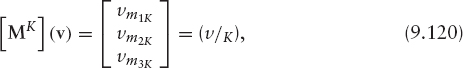
that is, matrix [Mk] selects among the set of all degrees of freedom v ∈ ![]() the three that correspond to the element K.
the three that correspond to the element K.
In that way, Problem 13 can be written as

Notice that this equality must be satisfied for all ![]() therefore,
therefore,

where

The 3 × 3 matrix ![]() is often called the elementary matrix, and the three-component vector
is often called the elementary matrix, and the three-component vector ![]() is the elementary right-hand side, corresponding to the element K.
is the elementary right-hand side, corresponding to the element K.
The operations in (9.122) are known with the name of assembling of the elementary matrix and the right-hand-side terms. Let us see how it works in practice. By definition,
Hence,
and therefore,
In that way, for the calculation of Ah and bh the following algorithm can be used:
- Initialize Ah and b to zero.
- Do a loop over the elements of Th. For every K ∈ Th, compute
 and
and  and then define

Change to the Reference Element The integrals that appear in the calculation of ![]() and
and ![]() will be done through a change of variable to the reference element. Integrals on the boundary and on the interior have to be dealt with differently. Therefore, we will denote
will be done through a change of variable to the reference element. Integrals on the boundary and on the interior have to be dealt with differently. Therefore, we will denote

and
Let ![]() be the triangle of vertices
be the triangle of vertices
that we will call the reference triangle. Let K be any element of Th. There exists a unique affine invertible mapping FK: ![]() → K such that
→ K such that ![]() for i = 1, 2, 3. It is the mapping
for i = 1, 2, 3. It is the mapping
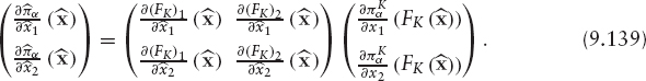
where CK is the matrix
It is easy to check that
where
Indeed, ![]() and also
and also ![]()
The formula of the change of variable is
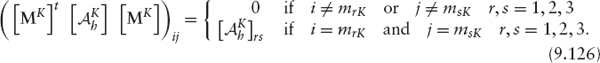
On the other hand, by the chain rule, we have that
Therefore,

or, in summarized form,
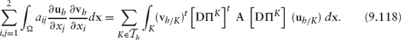
Substituting this expression for [DΠK] in (9.127) we obtain

If we introduce the following notation:
we may write

If the coefficients ![]() are constant in K, then [GK] is constant in K and
are constant in K, then [GK] is constant in K and

The numbers
do not depend on the element considered and are calculated just once. Also, notice that
In this way, just the matrix [GK] and, ![]() depend on the element. The matrix [GK] is worked out using the values of aij and the coordinates of vertex
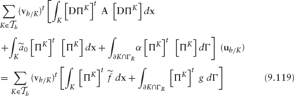
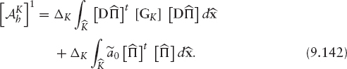
depend on the element. The matrix [GK] is worked out using the values of aij and the coordinates of vertex ![]() Completing the calculations described, we obtain
Completing the calculations described, we obtain


Similarly, for the right-hand-side term we have that
We proceed to compute the boundary integrals of the elementary matrix and the right-hand side by a change of variable to the reference element. In order to do so, we will define parameterizations of the edges of K
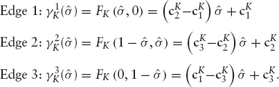
Therefore,

and finally we have

where
The calculation of the integrals that appear in ![]() as well as the ones that appear in the elementary matrix when the coefficients aij, and
as well as the ones that appear in the elementary matrix when the coefficients aij, and ![]() are not constant in the element K, are done via numerical integration. It can be shown ([180]) that the error does not increase if an appropriate formula, which depends on the finite element space, is used.
are not constant in the element K, are done via numerical integration. It can be shown ([180]) that the error does not increase if an appropriate formula, which depends on the finite element space, is used.
1 Research, VAR, risk management, pricing.
2 For example the convertible bond call provision or any other issuer callable contract.
3 In fact, the pointwise inequality holds
![]()
4 They use a characteristics/FE method for the space discretisation and the Brennan Schwartz algorithm to deal with the American early exercised.
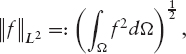
5 L2(Ω) is the space of square-integrable ![]() -valued functions defined in Ω with the norm
-valued functions defined in Ω with the norm
![]()
l∞(L2(Ω)) is the space of ![]() -valued functions, ψ, defined in
-valued functions, ψ, defined in ![]() such that ψ(tn) ∈ (Ω) for all n = 0, …, N. In this space we consider the norm
such that ψ(tn) ∈ (Ω) for all n = 0, …, N. In this space we consider the norm

6 Hk+1(Ω) is the Sobolev space of order k + 1. This is the set of ![]() -valued functions defined in Ω which are square-integrable and have square-integrable derivatives up to order k + 1. In this space we consider the norm
-valued functions defined in Ω which are square-integrable and have square-integrable derivatives up to order k + 1. In this space we consider the norm
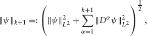
where Dα denotes the derivative of order α.
7 This issue has a call announcement period of 45 days and a conversion announcement period of 14 days. It has also the so-called French dividend conversion, meaning that the shares received upon conversion do not pay those dividends paid by ordinary shares between the date of conversion and the end of the fiscal year in which conversion occurs. All those features have been ignored for the sake of simplicity.
8 Both time series were obtained from Bloomberg.
9 For d = 3, those are edges, faces, and vertices.