CHAPTER 4

Hybrid Products

In this chapter we discuss when it is necessary to use stochastic rates to price a derivative and what effects they have on the prices, giving the conditional trigger swap TARN, convertible bond and exchangeable bond as examples.

All options depend on interest rates through the discounting of future payments. If we treat interest rates as stochastic, then the money market account (often used as our numeraire) becomes stochastic. So apart from the explicit hybrid products, where we receive payments based on both interest rate market observables (LIBOR and CMS rates) and equities, we may also need to consider stochastic interest rates when pricing options where the value of some equity/index affects the time when we receive some payments. A good example of this is the target redemption note (see section 4.3).

4.1 THE EFFECTS OF ASSUMING STOCHASTIC RATES

Whether or not we choose to price a particular option with stochastic rates will depend on what risks we think are significant and against which we need to hedge ourselves. Interest rates tend to be less volatile than equities, with typical short-rate volatilities being around a few percent, whereas equity volatilities may be of the order 10% to 100%. Often, the effect of stochastic rates will be swamped by the effects of the more volatile equities, and it will not be necessary to use a more CPU-intensive two-factor model.

Stochastic LIBOR and CMS rates The most obvious effect of stochastic interest rates is to make quantities such as LIBOR and CMS¹ rates stochastic. If we have an option with a payoff dependent on a combination of these and an equity performance, there is a good chance we will need to model the interest rates as stochastic. However, as mentioned, the interest rate volatilities may be so low as to make this unnecessary. Examples of derivatives that depend on stochastic interest rates in this way are conditional trigger swaps (see section 4.2) and hybrid best-of products, which pay coupons of the form

These derivatives tend to depend strongly on the assumed correlation between the interest rate and equity processes.

Note that derivatives containing a stream of LIBOR payments that cannot be terminated early do not necessarily need to be modeled using stochastic interest rates as we can hedge the payments in a way that does not depend on what happens to the LIBOR rates.²

Stochastic numeraires The second effect of assuming stochastic rates is to make the money market account and zero-coupon bond prices stochastic. These are often used as numeraires, so the time value of money is affected. Any option where the time of a given payment is uncertain will be affected by stochastic interest rates. Examples of such options are

• Bermudan/American callable options. Here the timing of the strike payment depends on when the holder decides to exercise; that decision will depend on what has happened to the interest rates.
• Target redemption notes (TARNs; see section 4.3) where the overall level of return is guaranteed, but how the return is distributed throughout the life of the option depends on an equity performance.
• Any option in which you receive a payment the first time an event happens (e.g., a barrier is breached).
• Any option with a stream of LIBOR payments that can be called/knocked out, such as the floating side of a conditional trigger swap.

The longer the maturity of an option, the greater will be the effect of stochastic rates. A 1% change in interest rates will have only a 1% effect on the price of a one-year zero-coupon bond, but the effect on the price of a 30-year bond will be compounded up to more like 30%. For this reason, many options will be considered to be hybrid options once their maturity becomes large enough, say five or ten years.

Adjusted local volatilities The final effect of stochastic rates that we will mention here is more subtle. It is not so much a direct effect of stochastic rates on the payoff of a product as a breakdown of our usual modeling assumptions for long-dated options. Interest rates affect the stock price process through the drift term; in the risk-neutral measure the drift of the stock price is just the short rate r_t. Ignoring dividends, we can write the stock price at time t as

where is the equity process volatility (which may be stochastic), W^S is the Brownian motion driving the stock price process in the risk-neutral measure and ε is the Doleans-Dade exponential.³

When we assume interest rates are deterministic, all of the volatility of the terminal stock price, S_t, comes from the final exponential in the above equation and so we calibrate to implied volatilities. In reality, since interest rates are stochastic, the first exponential in the above equation is also a source of randomness and so the equity process (local) volatility must be adjusted to match the implied volatility surface (for more details of this, see chapter 8). Note that this effect exists even when the interest rates are uncorrelated with the equity process. If we are always calibrating to market implied volatilities, the terminal stock price distribution in the t−forward measure (and thus the prices of European-style equity options) is unaffected by our assumptions about stochastic rates.⁴ However, options that are more directly sensitive to the local volatility than the implied volatility will be affected.

In particular, options with a knock-out feature will be affected. Consider an option that pays a fixed coupon c semiannually up to the first time the stock rises above some barrier B on one of the coupon dates, T_i. The probability of being above the barrier at time t (in the t−forward measure) is unaffected by our rate assumptions.⁵ However, the more positive the correlation between stochastic rates and the equity process, the less the equity local volatility will be and so the more correlated the stock prices on adjacent barrier dates will be.

We can write the present value of the coupon payment on date T_n as

This probability can be rewritten as

If the local volatility is reduced by introducing stochastic interest rates, the terms in the above expression will also be reduced as there is less volatility to allow the stock to move over the barrier at date T_i, given that it wasn't over the barrier at date T_i−1.

Note that the first exponential in equation (4.1) will be correlated with the short rate at time t, r_t. Even if there is no instantaneous correlation between the equity process and the interest rate process (i.e., dS and dr are uncorrelated), the terminal values (S_t and r_t) will be correlated, so derivatives with a payoff sensitive to this correlation will be affected by modeling rates as stochastic even if we assume no instantaneous correlation.

4.2 CONDITIONAL TRIGGER SWAPS

A conditional trigger swap is like a standard swap in that the holder (or issuer) receives coupons in exchange for paying LIBOR. However, what would normally be fixed coupons depend on the performance of an equity. Additionally, the whole trade knocks out if the equity ever goes above some barrier.

In each of the example trades here, the underlying is the Nikkei (N225) index and the payments are made in Japanese yen. The holder pays JPY LIBOR semiannually on dates T_i and receives c₁ at date T₁, then subsequently receives

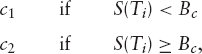
at date T_i where B_c is a barrier set below the current spot level. If the index performs well, the holder will receive a string of large coupons, whereas if the index plunges below the barrier, he will receive only the small coupons.

On top of this, the whole structure knocks out if the index goes above B_k on date T_i, where B_k is a knock-out barrier level set above the current spot. On the date when the structure knocks out, the LIBOR and coupon payments are still made, but subsequent ones are not.

The payoff is shown graphically in figure 4.1.

Without the knock-out barrier, this deal would not require stochastic rates at all. We can value the floating side payments as we normally would, as 1 − P(T₀, T_N). We can decompose the fixed side payments into the guaranteed amounts δc₁, where δ is the appropriate day-count fraction, and a series of digital options paying δ(c₂ − c₁) if S_Ti > B_c, which can be completely hedged with European options.

We can think of the floating side of the option as being equivalent to paying 1 at T₀ and receiving 1 at maturity or when the option knocks out. This is shown in figure 4.2. The floating side payments in the option are therefore sensitive to stochastic rates because the time when the holder effectively pays back the notional is stochastic. The value of the stream of LIBOR payments can be written as

FIGURE 4.1 Cash flows for a conditional trigger swap. T_f is the first observation date T_i at which S(T_i) > B_k or maturity.

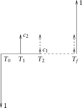
FIGURE 4.2 Alternative cash flows for a conditional trigger swap. T_f is the first observation date T_i at which S(T_i) > B_k or maturity.

For now we will ignore the effect of the stochastic rates on the distribution of the time T_f and just note that each of the terms

is positively correlated with interest rates. The more positively correlated the terms

FIGURE 4.3 Effect of correlation on the floating side of a sample of conditional trigger swaps. SR and DR refer to stochastic rates and deterministic rates, respectively.

are with interest rates, the greater each of the expectations will be. The greater the index/interest rate correlation, the less positively correlated the above terms will be with interest rates, and the smaller the PV of the LIBOR payments will become. As the correlation increases, the value of the floating side decreases.

The other effect to consider is the change in the local volatility. As correlation increases, the local volatility decreases and so the probability of the option's knocking out by a particular date decreases. Consequently, as correlation increases, the expected lifetime of the option (the expectation of T_f) increases. This is a smaller effect than the one discussed above, so is not noticeable in the floating side, but we can see that the PV of the fixed side payments do indeed increase slightly with correlation.

Figures 4.3 and 4.4 show the effect of correlation on the PV of the float and fixed side payments for some representative trades. Note that although the maturities of these deals are 15y or 30y, the expected lifetimes are actually much smaller, so the stochastic interest rates have only a small impact on the prices.

The details of the trades are as follows:

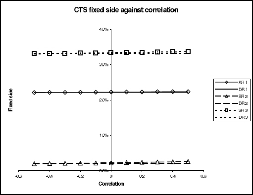
FIGURE 4.4 Effect of correlation on the fixed side of a sample of conditional trigger swaps. SR and DR refer to stochastic rates and deterministic rates, respectively.

4.3 TARGET REDEMPTION NOTES

4.3.1 Structure

The target redemption note (TARN) is a coupon-bearing, capital-guaranteed structure that pays an attractive coupon for the first year or two, and that furthermore pays a guaranteed⁶ total coupon amount, distributed among the remaining coupon dates of the structure. The structure's maturity might be eight years or more.

The defining features of the TARN structures we consider here are:

• The sum of coupons paid (TARN level) is guaranteed and the capital protected.
• For an initial period, coupon payments are fixed.
• The timing of the residual coupon and of the redemption payment are not guaranteed, but are dependent on the performance of an underlying.

So the market risk is in the timing of the payments, not in their aggregate size.

A wide variety of instruments can be used as the underlying for a TARN. The structure originated as an interest rate derivative: Equity-linked TARNs are a more recent development (since around 2003). Equity-linked underlyings can be indices (e.g., Dow Jones Euro Stoxx50), baskets (of as many as 20 stocks) or worst-of baskets (having just a few constituents in the basket, perhaps just three). A CPPI strategy (chapter 5) can also serve as the underlying for a TARN.

We will adopt a typical example TARN to study, with terms as follows:

• 10-year maturity.
• Underlying is the Dow Jones Euro Stoxx 50 index.
• TARN level of 13.5%.
• Annual coupons C_i,1≤i≤10 at anniversary dates t_i,1≤i≤10.
• The first two coupon amounts are fixed: C₁ = C₂ = 4.5%.

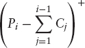
The remaining coupons are equity linked and given in terms of the performance of the underlying since the inception of the structure, P_i = S(t_i)/S(0) − 1, thus:

In words: The equity-linked coupons, before the last one, pay the excess of the stock's performance, up to the coupon date, over the accumulated coupons prior to that time; the total aggregated coupon being however capped at the TARN level. The final coupon “tops up” the total aggregated coupon to equal the TARN level irrespective of the underlying stock's performance.

When the total aggregated coupon reaches the TARN level, the capital is returned and the structure terminates. Neither the total income from the structure nor the repayment of capital is therefore in doubt: just the timing of the income and redemption payments, and hence the yield (to maturity or to early redemption). The structure attracts the investor who believes that it will be called early; say, after three or four years. In that case, he will have received attractive coupons from a medium-term note. He must believe that it is not unreasonable to suppose that the index will have risen by 13.5% in three or four years.

To illustrate the risk taken on this market view, we may look at the internal rate of return (IRR) arising from various possible redemption scenarios. Table 4.1 lists the most favorable scenario (which is that the instrument is called after just three years), the two extreme scenarios at four-year termination (the ones generating the minimum and maximum coupon at three years), the most favorable five-year termination case and the ten-year case. We note that even the most favorable four-year termination reduces the IRR by more than 1% and the most favorable five-year termination by nearly The investor's yield drops abruptly if his favorable early-termination scenarios are not realized. Worse still, if the market falls and does not recover, he is trapped in a structure that provides a yield far below risk free. A further conclusion from the table is that the dominant factor in the realized IRR is the timing of the redemption payment, not the details of how the coupon is distributed amongst the anniversary dates.

TABLE 4.1 Internal rates of return for TARN redemption scenarios

Compare also figures 4.10 and 4.11 showing how the TARN's value derives from the distribution of early- and late-termination cases.

While this is not an atypical structure, there are variants on the theme. One such caps each coupon payment, potentially preventing the TARN level being reached at some coupon date and thereby lengthening the structure when the basic TARN would have redeemed early. In the above expression for the coupon amounts,

is in this case replaced by

4.3.2 Back-Testing

For the purposes of marketing a structured derivative, it is common to perform back-testing. This procedure evaluates how the structure would have performed had it been purchased at some time in the past. In particular, it is common to evaluate the results of having, hypothetically, made the investment in the structure on each business day during an appropriate time interval, using historical daily time series for all relevant underlyings.⁷

Although back-testing is no part of derivative valuation, we apply it to our example TARN to illustrate some of its features. The Stoxx50 index is available from January 1987, so derivatives of ten-year maturity can be back-tested meaningfully, assuming one “clone” of the structure to be initiated per business day during the ten years between January 1, 1987, and December 31, 1996. It transpires that even the latest starting of the simulated structures would have terminated by December 31, 1999. Accordingly, we can calculate their realized IRRs and plot them: Figure 4.5 shows the realized IRR for each trial, and figure 4.6 shows their distribution into the maximum possible IRR and percent-wide bands below it.

FIGURE 4.5 Realized IRRs for each hypothetical back-tested TARN. One is assumed to have been started each business day for ten years from January 1, 1987.

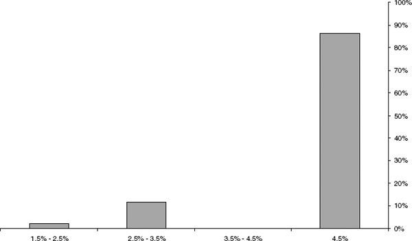
FIGURE 4.6 The distribution of realized IRRs for hypothetical back-tested TARNs. The gap in the histogram corresponds to the gap between the three-year termination case and the most favorable four-year case in the last row of Table 4.2.

We have the surprising result that 86% of the simulated TARN issues terminate after three years (the market rose at least 13.5%).

This is in fact a nice illustration of the power of back-testing: If the investor believes that this behavior is representative of the outcome for an investment he is considering, he will see the investment as extremely attractive. The risk-neutral probability of markets rising 13.5% in three years is, of course, nowhere near this high.

We may gain some intuition for this high percentage by observing the time series for the index over the relevant interval (see figure 4.7). The vertical lines in the graph mark the start date of the last simulated TARN, and its redemption date. (It is clear by inspection that it terminates after three years, and in fact no simulated TARN survives later than this.) We can see that the back-testing interval is dominated by rising markets and excludes (because even the latest-starting TARNs have terminated) the decline from the markets’ peak in 2000, hence the excellent back-testing performance of this structure.

Now we are in a position to understand how the TARN offers such an attractive early coupon and what the pitfall is. The early coupons are paid for by the probability that the capital will be tied up for a long time, earning no great return, in the event that the early redemption scenarios are not realized. The larger the initial coupon, the lower the probability of early redemption and the longer it will be necessary to lock up the capital in order to make the structure value work. In structuring a TARN, there is a balance to be struck between initial coupons sufficient to attract investors, the probability that early redemption will not happen, and the length of time for which the investor's capital will be locked up in the structure if it is not redeemed early.

FIGURE 4.7 Closing levels of Stoxx50 from January 1, 1987. The vertical lines mark the inception date of the latest simulated TARN and its redemption date.

In the following sections, we extract the risks embedded in the structure, and indicate how the various models in which the structure can be valued quantify these risks.

4.3.3 Valuation Approach

Apart from the initial fixed-coupon payments, the TARN embeds a strip of call spreads, where the lower strike depends on the past performance, and a payment of the redemption amount on the first anniversary on which the performance reaches the barrier (i.e., TARN level), 113.5% of initial spot in our example. Hence, we may investigate the interest rate risk, the embedded lookback call spreads, and the barrier risk.

Barrier Risk We first concentrate on the barrier risk at K = 113.5%S₀. The barrier in question pays the redemption amount as soon as the stock reaches K, or at maturity if the stock never reaches this level. A barrier can generally be seen as a limit of call spreads. As such, the impact of using a Black-Scholes-type model is severe: It neglects the presence of the skew around the barrier.

In formulae, this rests on the fact that

(Here denotes the implied Black-Scholes volatility of a call with strike K and the BS superscript indicates Black-Scholes-type formulae.) To illustrate the impact of the vega term, we may evaluate the digital in the Black-Scholes Model and compare it with approximations to the derivative of the call price using call spreads of ±∈ around the barrier K.⁸

The results of this test for the digital at 18-month maturity are given in Table 4.2. (Compare also figure 1.5, in which similar comparisons are illustrated.)

The wide discrepancy here forces us to use a model that takes into account the skew, such as local volatility. In principle, such models reprice all European vanillas correctly. Consequently, as we can see in Table 4.3, they give consistent prices for the barriers. (Again, compare figure 1.5.)

TABLE 4.2 The Black-Scholes digital compared to call spread approximations

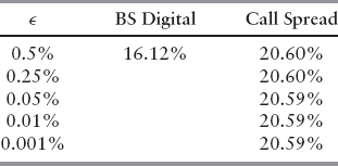
TABLE 4.3 The Black-Scholes digital compared to call spread approximations and local volatility prices at various maturities. Data for Stoxx50, June 2005

Lookback Elements The next elements for consideration in the TARN are the embedded call spreads. The coupons have the form:

which shows that later coupons are lookback-type call spreads.⁹ In general, such structures might depend strongly on future skew and interdependency between the increments S_i/S₀ and S_i−1/S₀. Such effects are not always well captured by local volatility models.

To assess the impact of using a “structural” model (as opposed to a “fitting” model like local volatility) that still fits the European prices along the barrier K well, but that also has self-consistent implied volatility dynamics, we calibrate a Heston-type extended stochastic volatility model to the market. Carrying out the comparison between these two models and plain Black-Scholes and the call spread yields the comparison in figure 4.8 for the 113.5% barrier of our example. The same comparison for the TARN using a BS model (i.e., term structure of implied volatility along K), a local volatility model and a stochastic volatility model is shown in figure 4.9.

The TARN can be thought of as two guaranteed coupons of 4.5%, plus an option to receive the notional when a barrier of 13.5% is reached, plus an extra 4.5% paid somewhere between year 3 and year 10. Well-calibrated stochastic or local volatility models should agree on the prices of the fixed coupons and the barrier option, as well as the value of the first variable coupon. It is only the remainder of the deal that behaves like the sum of lookback options (and then only if the index falls within the narrow range of 109% to 113.5%). It is perhaps not too surprising that the choice of the stochastic versus local volatility model does not have a large effect on the price.

Impact of Stochastic Rates Although there is no explicit dependence on interest rates in this product, the choice of deterministic versus stochastic rate models and of the correlation between the index and the rates can still have a significant effect on the price.

This behavior can be understood from looking at figures 4.10 and 4.11, where we show the probabilities of the TARN expiring at a particular date and the corresponding contributions to the overall price.

As the correlation between the index and the rates is increased, two effects occur:

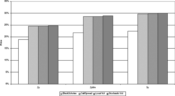
FIGURE 4.8 Different models applied to the 113.5% barrier option of various maturities.

• The local volatility of the index process has to decrease (as the effect of the stochastic rates on the implied volatilities becomes stronger).
• The cash bond becomes more positively correlated with the index level.

The first effect increases the correlation between the index prices on consecutive fixing dates, which increases the probability that if the index is above the barrier on date i, then it was also above the barrier on date i − 1. The probability of the TARN expiring in each of periods 4 to 9 is therefore reduced (figure 4.10). The second effect means that paths where the index performed badly (and so the TARN expired after ten years) have a smaller cash bond and so the final payment in less strongly discounted and so worth more, seen from today. This can be seen from figure 4.11, where the correlation has a very large effect on the contribution to the TARN price of the paths expiring after ten years. Note that the second effect becomes more pronounced for later maturities thanks to compounding up of the cash bond. The net effect is that the TARN value increases with increasing index versus rate correlation, as shown in figure 4.12.

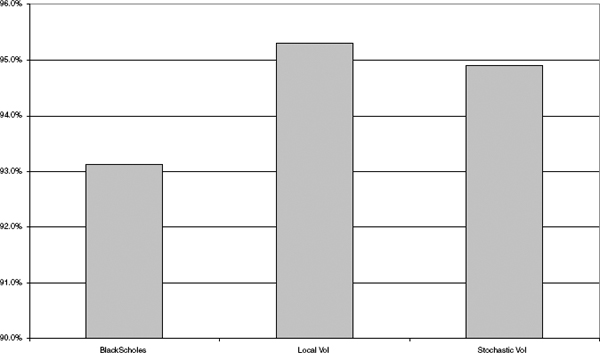
FIGURE 4.9 Different models applied to the TARN structure.

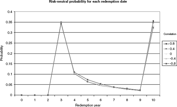
FIGURE 4.10 Risk-neutral probabilities of redemption on the possible expiry dates.

FIGURE 4.11 Contributions to the TARN value from the possible expiry dates.

4.3.4 Hedging

Once the deal is priced, a hedging strategy to manage the risk must be employed. The considerations necessary to hedge the product are similar to the pricing considerations: We are faced with some fixed coupons (for which we do not need any hedging), a barrier, and a stream of lookback call spreads.

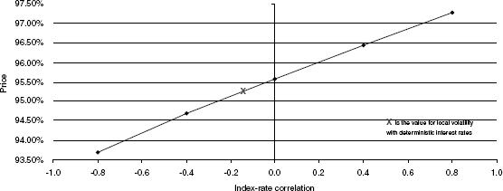
FIGURE 4.12 The effect on the calculated TARN value of correlation between the index and the EUR short rate, in a local volatility model with stochastic short rates.

Barrier Hedging The risk in hedging a barrier is that the delta becomes very large when we approach the barrier, and suddenly collapses when the barrier is reached. We then face the problem of not being able to unwind our delta position fast enough and face a gap risk. To alleviate the situation, call spreads can be used to approximate the barrier. However, the size of the call spread is crucial: set too large, the product becomes too expensive; too low, and the gap risk becomes too strong. In general, the size of the spread lies in the experience of the trader and depends on the liquidity of the stock, the size of the position, any other positions in the book, and so forth.

Lookback Call Spreads The specific nature of the lookback call-spreads embedded in the TARN is that the payment of one spread determines the lower strike of the preceding call.

One possible strategy is therefore to set up call spreads for all times t_i: i ≥ 3 with upper strike K (the barrier) and lower strike initially at 109%S₀. The later strikes might also be adjusted by the probabilities of the process reaching the barrier up to t_i. Clearly, this initial portfolio of calls must be adjusted during the life of the trade to account for the actual movement of the stock, taking into account the transaction costs for each repositioning.

4.4 CONVERTIBLE BONDS

4.4.1 Introduction

In this chapter we consider an intensity-based framework for pricing convertible bonds (CBs; see, for example, Overhaus et al. [31]) in a “two-and-a half-factor” setting. The two factors are the stock price and the interest rate. The hazard rate (the half factor) is modeled as a deterministic function of the stock, the interest rate, and time. We account explicitly for the stock price behavior and holder's rights in the event of default as well as the recovery value of the bond. Most comparable existing models are special cases of this general setting.

There are three main issues on the modeling side:

• Whether the stock value or the firm value is the main underlying factor
• Whether there are additional stochastic factors, such as an interest rate or hazard rate
• How default is modeled and what happens upon default to the state variables, the CB holders’ rights, and the convertible value.

In general, credit risk models fall into two main categories: structural and reduced form (see Chapter 6). In structural models (see [72]–[82]) the state variable is usually the value of the firm or firm asset value, which moves randomly. All claims on the firm's value are modeled as derivative securities with the firm value as the underlying. Default occurs when the value of the firm hits or crosses a boundary. It is necessary to specify the process for the firm value, the location of the barrier, and the form and amount of recovery upon default. These models provide a link between the equity and debt instruments issued by a firm, which may be necessary, for example, in the valuation of CBs and callable bonds; they can be used, at least in theory, to optimize the capital structure, and default risk is endogenized and measured based on the share price and fundamental data only. However, the firm value is unobservable and often difficult to model. The volatility of the firm value is particularly hard to estimate. Also, models become too complex for reasonable capital structures. Finally, they are not well suited for pricing and hedging of credit instruments. In reduced form models (see [77], [83]–[88]) default is exogenous, occurring at the first jump time τ of a counting process, N_t, with jump intensity λ_t. The main issues in reduced form models are the specification of processes for the riskless short rate r_t, the hazard rate λ_t, and the recovery value.

The early models of convertible bonds (Ingersoll [89] and Brennan and Schwartz [90]) follow Merton [73] in using the value of the firm with geometric Brownian motion as the sole state variable. Brennan and Schwartz [91] and more recently Nyborg [92] and Carayannopoulos [93] included in addition a stochastic interest rate. Brennan and Schwartz and Nyborg assumed the short rate follows a mean-reverting log-normal process; Carayannopoulos assumed the short rate follows the Cox, Ingersoll, and Ross [94] model. Default risk is usually incorporated structurally by capping payouts to the bond by the value of the firm.

Recent literature, on the other hand, mainly uses the stock price as a state variable and either ignores credit risk (Zhu and Sun [95]; Epstein, Wilmott, and Haber [96]; Barone-Adesi, Bermúdez, and Hatgioannides [97]; Bermúdez, and Nogueiras [107]), incorporates it via a credit spread (McConnell and Schwartz [99], Cheung and Nelken [100], Ho and Pfeffer [101]), or models it in a reduced form setting as an exogenously specified default process (see Duffie and Singleton [87]). However, some authors have pointed out (see Schonbucher [102]) that given the hybrid nature of convertibles, asset-based models are the right class to consider in order to account for credit risk. Arvanitis and Gregory [103] implemented and compared both type of models for CB valuation. Bermúdez and Webber [104] proposed an asset-based model that incorporates both endogenous and exogenous default, as well as endogenized recovery.

In the equity-based approach most authors use a single-factor model, although some allow interest rates to be stochastic in addition. The Vasicek [105] or else the extended Vasicek (Hull and White [106]) model is used by Epstein, Haber, and Wilmott [96]; Barone-Adesi, Bermúdez, and Hatgioannides [97], Bermúdez and Nogueiras [107]; and Davis and Lischka [108]. Ho and Pfeffer [101] used the Black, Derman, and Toy [109] model; and Zvan, Forsyth, and Vetzal [110] and Yigitbasioglu [111] used the Cox, Ingersoll, and Ross [94] model. Cheung and Nelken [112] adopted the model developed by Kalotay, Williams, and Fabozzi [113].

Very few authors model the hazard rate stochastically (Davis and Lischka [108], Arvanitis and Gregory [103]). Most recent papers model the hazard rate as a deterministic function of the state variables (also called a quasi-factor or half factor) instead. To model the credit spread as a function of the state variables is very intuitive and appears to provide realistic valuations, sensitivities, and implied parameters, but it does constrain the credit spread to have an explicit relationship with the stock price. This suggests developing a model in which both stock prices and credit spreads follow separate but correlated random processes, as proposed by Davis and Lischka [108]. As these authors point out, although there are three sources of uncertainty—stock price, interest rate and credit spread—more than two factors tend to be avoided for computational tractability. From the implementation point of view, stochastic hazard rates offer the same complexity as stochastic interest rates, given that the dynamics for both processes are often very similar and their role in the valuation PDE is analogous (Duffie and Singleton [87]).

The first authors to have modeled default exogenously, in the spirit of reduced form models, were Davis and Lischka [108] (DL) and later Takahashi, Kobayahashi, and Nakagawa [114] (TKN). They assumed that default occurs at the first jump of a Poisson process, and they modeled the intensity of the jump as a deterministic function of the stock price. They assumed that upon default the stock price jumps to zero. DL modeled the recovery as a constant fraction R of the par value of the bond, whereas TKN modeled recovery as a fraction of the market value of the bond prior to default. However, it can be argued that these approaches penalize the equity upside of the CB. The value of a convertible bond has components of different default risk; the value contributed to the bond by its conversion rights can be argued not to be subject to the same risk treatment as the fixed payments. Therefore, it may be convenient, or even essential, to split the CB value into a bond part and an equity part. In general, the value of the debt and equity components will be linked, and the valuation problem reduces to solving a coupled system of equations. Splitting models allow one to apply a different credit regime to the debt and equity components. Moreover, they may be of interest to investors in order to identify different sources of risk and be able to hedge them. How to split the convertible value, though, is an open and controversial matter.

The first authors presenting splitting and writing the model as a coupled system of equations were Tsiveriotis and Fernandes [115] (TF). The value of the equity component and the value of the bond component were discounted differently to reflect their supposed different credit risk. Ayache, Forsyth, and Vetzal [116], [117] (AFV) extended previous literature by proposing a general specification of default in which the stock price jumps by a given percentage η upon default and the issuer has the right either to convert or to recover a given fraction R of the bond part of the convertible. The way they define the bond part is different from the original definition of Tsiveriotis and Fernandes.

We consider a unified framework for pricing convertible bonds incorporating interest rate and credit risk. We assume a jump-diffusion process for the stock price and a mean-reverting process for the interest rate. We model the intensity as a deterministic function of the stock and the interest rate, leading to an extra so-called quasi-factor or half factor. Upon default, the model has an arbitrary loss rate η on the stock price, and an arbitrary default value V^* for the convertible that may be a function of the state variables. The model contains many other models as special cases. We identify most of the previous models, and we show that the main difference between them is the specification of the recovery value.

DL and TKN implement their model in a lattice. TF use explicit finite differences and an explicit algorithm to solve the coupled system of equations. AFV use a modified Crank-Nicolson method combined with a penalty method for the free boundaries and an implicit algorithm to solve the coupled system of equations. In chapter 9 we discretize using a Lagrange-Galerkin method, and use an iterative method to deal with the free boundaries.

In the next section we present the general valuation framework. Section 4.4.3 provides a detailed specification of the model, namely the interest rate model, the hazard rate, the recovery value, and the conversion rights upon default. Also in this section, previous models that are special cases of the general framework are identified. Section 4.4.4 provides the analytical solution for a special bond convertible just at expiry.

4.4.2 The Governing Equation

We follow a standard procedure given, for instance, by Protter [118]. Suppose that the value S_t of the underlying asset follows a jump-augmented geometric Brownian motion under the objective measure, P^*,

where is a standard Brownian motion under P^*, d_t is the continuous dividend yield, and q_t is the repo rate. N_t is a counting process with intensity η_t is a deterministic loss rate. N_t models exogenous default events. At a jump time τ for N_t the equity value falls by a proportion η_τ,

It is well known that the process is the P^*−compensator of N_t, that is, the unique finite-variation previsible process such that is a martingale under P^*.

Under the equivalent martingale measure (EMM), P, associated with the money market account, the relative price is a martingale, so

where is a standard Brownian motion under P and ν(dt) = λ_tdt is the P−compensator of the jump component.

Notice that the setup defined by equation (4.4) is an incomplete market, meaning that there is at least one contingent claim that cannot be hedged. Equivalently, under the assumption of no arbitrage, there is no unique equivalent martingale measure with which to price a contingent claim. However, given that the loss rate, η_t, is deterministic, the market can be completed by adding a defaultable bond issued by the firm whose equity is modeled by S_t.

Let us also assume that the short rate follows the stochastic process

where μ_r and σ_r are the expected rate of return and volatility of the spot interest rate, which may be functions of the short-rate level as well as time. and are both Brownian motions that may be correlated

We suppose that the firm has issued a convertible bond with market value V_t. The bond matures at time T with face value F. At any time up to and including time T the bond may be converted to equity. Its value upon conversion at time t is n_tS_t, where n_t is the conversion ratio (which may be zero). The bond may be called by the issuer for a call price M_Ct and also it may be redeemed by the holder for a put price M_Pt. We assume that call and put prices include already accrued interest, which must be paid by the issuer upon call and upon put.

By Ito's lemma (see Jacod and Shiryaev [119]), the process followed by V_t is

where and is the value of the convertible bond if a jump occurs at time t.

Under the EMM the relative price is a martingale. Imposing this condition, we have

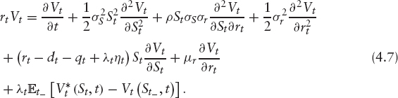
Notice that dt is the compensator of the jump ΔV(S_t−. When is a deterministic function of S_t = S_t−(1 − η_t), equation (4.7) reduces to

Inequality constraints that follow from the optimal conversion, redemption, and call strategies, as defined by Brennan and Schwartz [90], make the convertible bond valuation problem a free-boundary problem that can be formulated as a variational inequality. This is modeled below via a Lagrange multiplier p, which adds or subtracts value to ensure that the constraints are being met.

We will use the notation:

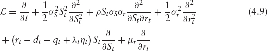
to write the valuation equation in short as

together with conditions

If the bond pays coupons discretely, typically every year or half year, let K(r_t, t_c)¹⁰ be the amount of discrete coupon paid on date t_c. Then the following condition must be imposed in order to avoid arbitrage opportunities:

Such discrete cash flows may be incorporated in the governing valuation equation by adding a Dirac delta function term − Kδ(t − t_c) to the RHS of (4.10).

The final condition for the convertible bond is the exercise condition at the maturity time T,

where we have introduced the adjusted face value

Solving (4.10) − (4.14) subject to boundary, final, and jump conditions gives the theoretical value of the convertible bond.

Splitting Procedures Given the hybrid nature of convertibles, it is possible and often desirable to split the value V of the convertible into a bond part W and an equity part U. Early models valued CBs by replication as a portfolio of a bond and a warrant. Unfortunately, this approach is limited to the case when the bond is convertible only at expiry and there are no other embedded options, such as call and put features. In general, the two parts are linked and the valuation problem is a coupled system of equations. Splitting models allows a different credit treatment to be applied to the debt and equity parts. This may be of interest to investors in order to identify their risks and be able to hedge them.

Let us assume the value of the bond is split into an equity part U and a bond part W. U is the part related to payments in equity, and therefore includes the conversion and call option. W is related to payments in cash, and includes the coupons and the put option. In general, both are derivatives on the underlying stock price and the instantaneous interest rate, and will follow partial differential equations similar to (4.10) with default values given by W^* and U^*, respectively. The two parts have embedded early exercise features and therefore follow inequalities with Lagrange multipliers p^W and p^U,

To be fully specified we need to supply inequality constraints and final conditions to (4.17) and (4.18). At the final time the payoff to the convertible is given by (4.16).

The splitting determines how V_T is allocated between W_T and U_T. How to decompose the convertible value, or equivalently how to define the bond and equity parts, is an open and controversial matter. Three possible splittings are (see figure 4.13):

• Splitting 1. U_T: asset or nothing call, W_T: cash or nothing put
• Splitting 2. U_T: equity, W_T: equity premium (put)
• Splitting 3. U_T: risk premium (warrant), W_T: bond floor

The motivation of the splitting is to apply a different credit treatment to equity and debt. Originally, in the TF model, the main objective was to use a different discount factor for the debt part and the equity part, such that the bond part is discounted with the risky rate and the equity part with the risk-free rate. The same effect may be achieved without the splitting by modeling the hazard rate as a function of the stock price. However, if we want to use a different recovery in bond and equity, a splitting is necessary in order to define the recovery value of the convertible. It will be mandatory to solve a coupled system of equations only when the default value of the convertible V^* depends explicitly on one or both of the values of the equity part U and the bond part W.

4.4.3 Detailed Specification of the Model

In this section we discuss in detail the remaining components of the model, namely the hazard-rate specification, the recovery value, and the conversion rights upon default.

FIGURE 4.13 Possible splittings of the CB payoff at maturity.

TABLE 4.4 Models for the hazard rate

Davis and Lischka [108]	λt
Olsen [120] Takahasi, Kobayahashi, and Nakagawa [114] Ayache, Forsyth, and Vetzal [117]	c + k/Sa
Arvanitis and Gregory [103]	k exp [−aSt + d]
Das and Sundaram [121]	k exp [brt + c(T − t) + d]/Sa

The Hazard-Rate Process As an alternative to stochastic hazard rate (chapter 3, Davis and Lischka [108]), herein we may use a deterministic function of the state variables and time. Many parameterizations could be applied; Table 4.4 shows some specifications that have been used in the literature. Several authors model the hazard rate as a function of the stock price only, and impose negative correlation via a power or an exponential function. In both specifications the spread is a monotonic decreasing function of the stock price; but only the power function guarantees an infinite hazard rate for zero stock price, which may be a desirable property (see Olsen [120]). Recently Das and Sundaram [121] have combined an exponential dependency on the interest rate with a power dependency on the stock price, and have added the time to maturity. They calibrated the hazard rate using market prices of CDSs and historical data, and they tested this approach empirically by pricing some real convertible bonds. Their results seem very satisfactory. Andersen and Buffum [122] are concerned with the simultaneous calibration of the hazard rates and the volatility smiles; they point out the need to make the hazard rate time dependent to avoid mispricing.

The Recovery Value Regarding the recovery of defaultable claims, many models (as reviewed by Schonbucher [102] and Bielecki and Rutowski [124]) have been proposed in the literature: recovery of treasury (RT), recovery of par (RP), multiple defaults (MD), recovery of market value (RMV), zero recovery (ZR) and stochastic recovery.

The RT is very convenient from the computational point of view. The reason is that the price of a defaultable issue under RT is a weighted average of the default-free instrument and the price under zero recovery, which is usually easy to compute. However, the RT can lead to unrealistic shapes of spread curves and lead to recoveries above 100%. The RP and RMV models are similar for issues close to par. The RMV is more consistent for the pricing of credit risk derivatives, but it does less well in pricing downgraded and distressed debt. The RMV is very elegant, in the sense that pricing of financial instruments can be done by discounting with the adjusted defaultable rate r + λ(1 − R), where λ is the hazard rate and R is the recovery rate. In RP the pricing is more complicated. Both models are suited for the calibration of the implied credit spreads, although in RMV it is not possible to separate the calibration of the hazard rate, λ, and the loss rate, (1 − R). RMV cannot be used with firm-value models, whereas the RP can be used in intensity-based and firm-value models. Finally, the intuition behind both models is different: the RMV is motivated by the idea of reorganization and renegotiation of debts; the RP is motivated by the idea of bankruptcy proceedings under an authority ensuring strict relative priority.

Suppose default occurs at time τ. We define the recovery value on the CB, V^*, as the sum of the recovery values on the bond and equity parts, W^* and U^*, respectively,

Conversion Rights upon Default Another issue regarding the default value is whether or not the model should allow for conversion upon default. Realdon [129] showed that it can be rational for CB holders to convert when the debtor approaches distress. In the pricing literature, only AFV allow for conversion upon default. This is consistent with the assumption that the stock price falls on default by a given fraction η and does not necessarily vanish. We adopt their assumption and redefine the bond value upon default as the maximum between the conversion price and the recovery value. In this case the pricing equations can be written as

No other models explicitly consider holder rights on default. However, given that DL and TKN assume the stock price jumps to zero upon default, the conversion option is worthless.

Previous Models as Special Cases of General Framework Most of the previous models fit into the general framework presented above. The particular specification of the hazard rate, the loss rate, and the recovery value will determine the difference. We have summarized why in Table 4.5.

• Davis and Lischka

Their equation is a special case of (4.10) for deterministic interest rate, loss rate η equal to 1, and recovery of par.

• Takahasi, Kobayahashi, and Nakagawa

Their equation is a special case of (4.10) for deterministic interest rate, loss rate η equal to 1, and recovery of market value.

• Tsiveriotis and Fernandes

TABLE 4.5 Comparison of previous models

Although TF do not discuss default, and they model credit risk via a credit spread, a posteriori we could identify their model in the more general setting of the previous section. The equation they propose for the total value of the convertible is the one-factor counterpart of (4.10) for zero loss rate, η, constant hazard rate, λ, equal to the credit spread, r_c, and value upon default, V^*, equal to the equity part of the bond, U,

This means that in the event of default the stock price does not jump. Also the bond part vanishes, and therefore the holder is not entitled to any cash flows, but conversion is allowed at any time after default. This was pointed out by AFV.

We would rather give the following interpretation. If we write the credit spread, r_c, as the product of a hazard rate, λ, and a loss rate 1 − R, where R is the recovery rate on the bond part, it can be easily shown that the default value of the convertible turns out to be This means that on default the total equity part is recovered, which is consistent with the fact that the stock price does not jump on default, or equivalently the recovery on equity is one. On the other hand, the recovery on the bond part is not zero. Therefore, TF can be seen as a special case of (4.10) with zero loss rate η and recovery a fraction of bond and equity part.

4.4.4 Analytical Solutions for a Special CB

We consider a special case for which an analytical solution is available: a zero coupon bond, which is convertible only at expiry. It is well known that the value of such a convertible may be written as the sum of the value of the straight bond plus n call options on the underlying stock with strike price X = F/n. Indeed

For simplicity, we assume the default value on the bond, V^*, is independent of the state variables, although it may depend on time. This includes, for example, the RP and RT models. Closed-form solution under other recovery models can easily be found. The value of the convertible may be written as

where

• Z (r, t; s) is the Vasicek discount factor from time t to time s
• SV (t, s) is the survival probability of the issuer from time t to time s
• And

with

4.5 EXCHANGEABLE BONDS

The valuation of convertible bonds (CBs) under stochastic short-rate models and deterministic hazard rates is well established. In this section we introduce a minor extension that nevertheless introduces an interesting new feature.

We consider the case of a bond that is convertible into stock at the option of the holder, exactly as for a standard CB, but which is issued by an issuer other than the company into whose stock the bond is convertible. Such instruments are known as exchangeable bonds.¹¹ A typical use of this latter structure is for a company to issue bonds convertible into shares of another company in which it already has a stake, thereby reducing its exposure to that stock, and effectively selling its stake in the event that the bond is converted.

The principal new feature for modeling that arises here is the exposure to two credits. The company whose stock underlies the bond can default, or the issuer can default, and the consequences for the bondholder of these two possible defaults are quite different. We do not consider here any correlation between the defaults.

4.5.1 The Valuation PDE

We use the following diffusion processes for the equity and short rate processes:

where

• r_t is the instantaneous short rate, modeled as a Vasicek process (section 3.3.1).
• is the volatility of the share, which requires calibration as in chapter 8.
• N_t is a Poisson process with a deterministic intensity (hazard-rate function).
• θ_t and κ_t are the long-term mean and mean reversion speed, respectively.
• is the volatility of the short rate.
• and are correlated Wiener processes.
• N_t models exogenous default events of the company that issued the stock. At a jump time for N_t, the share price is assumed to fall to zero.

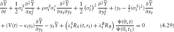
Let V(S_t, r_t, t) be the price of an exchangeable bond. Since V is subject to two sources of default risk, the issuer and the underlying risk, we introduce for the deterministic hazard rate function of the issuer. V(S_t, r_t, t) then satisfies the following PDE:

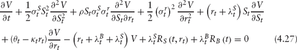
In (4.27) we introduce the following quantities:

• R_B(t) is the value recovered by the holder in case of default of the issuer: The “recovery value” of the exchangeable bond. We may decompose this value a little, thus

  

  in which

  — LP is the liquidation proceeds: the amount eventually received by the holder, delayed perhaps some while after the default event, by an interval known as the time to liquidation proceeds.

  — TLP is the time to liquidation proceeds: the interval that elapses, or is assumed to elapse for modeling purposes, between the default and the eventual payment of the liquidation proceeds.

  — P(t, t + TLP) is the discount factor from the default time t to t + TLP.

  The liquidation proceeds may in turn be broken down thus:

  

  in which

  — PP is the principal payable: the amount due to bondholders in the event of default. It could in principle be a function of time (Original Issue Discount bonds, zero coupon bonds issued at a large discount to par, might have this feature) but will typically be the full notional.

  — RR is the recovery rate: the fraction of the amount due to a bondholder which the issuer actually pays (or, again, is assumed to pay for the purposes of modelling).

  — The accrued is of course the amount accrued, at the time of default, on the coupon accruing at that time.

• R_S(t, r_t) is the value of the exchangeable bond if the underlying defaults. After the underlying defaults, the exchangeable loses all its equity value (the value due to the holder's conversion right), but the issuer is still obliged to make the coupon and redemption payments. Accordingly, the residue is simply an ordinary bond, although it retains its issuer call feature.

  However, the call feature will not have any value once the stock price has dropped to zero: if it is a soft call, then the trigger level will manifestly not be satisfied, and if not, then the call price would, in practice, be set sufficiently high as not to terminate the pure bond without equity content. Hence, R_S(t, r_t) can be approximated by the price of a standard coupon-bearing bond under Vasicek interest rates. Note that this is a risky bond, subject to default of the issuer, with recovery value equal to R_B. The closed-form solution for such a bond is given by

  

  where

  — i = 1, …, N runs over the remaining coupons.

  — K_i is the coupon amount payable at t_i.

  — SV^B (t, t_i) is the survival probability of the issuer from t to t_i.

  — P(r, t, t_i) is the zero-coupon bond price seen at time t and maturing at t_i, given r.

  — N is the notional.

  — R is the redemption factor (generally equal to 1, but greater than 1 for premium redemption bonds).

  — RV(r, t) is the expected value of recovery in case of default of the issuer as of time t.

This function depends on time t and the state variable r, so it needs to be evaluated at every node in the FD grid. The recovery contribution to the value of the bond, RV(r, t), is given by

4.5.2 Coordinate Transformations for Numerical Solution

In order to use (4.27) directly, the drift term θ_t is needed. The expression for this function involves second derivatives of P(0, t), so a piecewise linear function for P(0, t) (or the yield R(0, t)) is not sufficiently smooth. We can transform the problem such that θ_t, or first derivatives of P(0, t), are not required. In this we follow section 3.3.1.

The variable

is introduced. This follows the process

where Σ(t) is the variance of r_t

and

Since f(0, t) is the expected future short rate in the t−forward measure, PDE grids that remain centered on y_t = 0 will always capture the relevant region.

The process for the equity becomes

which contains the possibly nonsmooth functions f(0, t) and To remove this, we use the variable

where SV^S(0, t) is the survival probability of the underlying stock, given by

We have the processes

If V(S_t, r_t, t) = X(x, y, t) the pricing PDE in terms of the x-y variables becomes

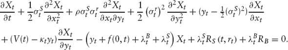
This has removed second derivatives of the yield curve (θ_t), and f(0, t) and from the convection (drift) term. However, the PDE still contains f(0, t), and in the reaction (discounting) term. To remove those (and improve convergence in the event of discontinuous forward or hazard rates), we can solve for a deterministically risky discounted form of X, that is,

where

This follows the PDE

In practice, at every time step from time t₁ to time t₂, with t₂ < t₁, we solve for the function

Notice that, at a known time step, t₁, we have

In particular, at maturity

therefore, solving for we do not need to rescale the payoff. The PDE for becomes

where

After solving this equation between two times t₁ and t₂, we can multiply by the risky discount factor between these two times

This is equivalent to solving for X(x, y, t).

Local Volatility The implied volatility of a European option is affected by both equity volatility and interest rate volatility, and the calibration of the equity local volatility needs to take this into account as described in chapter 8, alongside the possible jump to zero of the stock. This done, the algorithm will correctly reprice European options in the presence of deterministic default.

Implementation The recovery of the exchangeable R_B(t) in the event of issuer default is a function only of time if the time to liquidation proceeds is assumed to be zero. Otherwise, it is an approximation to drop the r-dependence. (The same calculation appears in the evaluation of a CB in a deterministic interest rate model, and in the valuation of a straight defaultable bond with recovery in a similar model.)

The value of the exchangeable bond at the time the underlying defaults R_S(t, r_t) enters the PDE (4.29) alongside R_B(t) in the source term

This quantity is evaluated at every point on the r-grid, at every time step.

An Example To make the discussion less abstract, we can consider a real example. In 2004, Banca Monte Dei Paschi Di Siena S.p.a. (Banca MPS) issued a bond convertible into the stock of Banca Nazionale Del Lavoro S.p.a. (BNL). Both are Italian banks listed on the Milan exchange¹²; the former is the world's oldest bank and the latter one of Italy's largest banking groups. Both are, unsurprisingly, good credits: as of late 2005, 5-year Banca MPS credit default swaps traded below 20 bps (basis points), rising to around 25 at ten years; five-year BNL credit default swaps traded around 35 bps, rising to 45 at ten years.

The exchangeable bond in question matures in July 2009; carries a 1% coupon, payable annually; and is convertible at any time after January 15, 2006, and callable by Banca MPS after July 2007, subject to the stock trading above €3.09 for 20 out of the preceding 30 business days. We can compare the valuations obtained for this bond with a hypothetical bond issued by BNL (a marginally worse credit) on its own stock; i.e., a standard convertible. Thus we keep the equity details unchanged in the comparison. Moreover, as the hazard rate appearing in the ∂/∂S term in (4.27) is that of BNL, the stock drift term is itself unaltered in the comparison.

We also make a recovery assumption: for illustration, we will assume recovery ratios of zero and 30% on default of the issuer. (In the exchangeable case, the separate default of the stock does not need a recovery assumption.) The comparison is shown in figure 4.14. The better credit of Banca MPS naturally tends to raise the fair price for the exchangeable. We should also bear in mind that the issuer being Banca MPS rather than BNL itself softens the effect of a potential default of BNL, as in the exchangeable case such a default would yield the full value of the coupon-bearing bond to the holder rather than, say, 30% of notional, which would be the case if the issuer were BNL.

FIGURE 4.14 Prices of exchangeable and hypothetical plain convertible bonds in percent of notional, for zero and 30% recovery assumptions.