CHAPTER 10

American Monte Carlo

10.1 INTRODUCTION

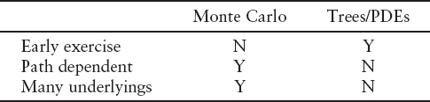
Traditionally, the numerical techniques for pricing derivatives fall into two distinct categories: Monte Carlo simulation and backwards induction methods such as trees or PDE methods. The following table sums up the strengths of each type:

In the most general terms, a derivative consists of a series of payments that depend on decisions made by the two parties in the contract and the values of some quantities observable in the market: the underlyings, which we will model with some stochastic processes. The payments can depend on the values of the underlyings observed on the date of the payment or on some functional of the paths followed by the underlyings up to the payment date.

To price derivatives using PDE methods, we must be able to represent the price of the derivative at time t as a function of a small number of state variables. For path-dependent options, the number of state variables may be larger than the number of underlyings. For instance, were we pricing an Asian option, our state-space at time t would have to include the current stock price and the running average stock price.

If we assume that our stock price follows the Black-Scholes SDE, and that the average is defined as

for some set of averaging dates t_i, then we have the following PDE for the price of the derivative in between averaging dates.

Across averaging dates we have the condition

where

At the maturity of the option, we calculate the final payment as a function of both S and A, suitably discretized, then evolve it back to the previous averaging date using equation (10.1). At that date, we can calculate the value of the option as a function of S and A before the averaging using equations (10.2) and (10.3).

The computational time taken to price derivatives using PDE methods scales exponentially with the number of state variables. For this reason, PDEs are not generally used to price options that depend on more than a few underlyings, or path-dependent options more complicated than simple knock-in/out barriers. For these options, Monte Carlo methods have traditionally been used.

In Monte Carlo pricing, we exploit the fact that the value of a series of payments, C_i at times t_i, can be written as

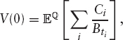
where B_t is the money market account and is the risk-neutral measure. We generate sample paths for the underlying processes and calculate the value the derivative would have if each path were realized. We then average over the paths to get the value of the option. We can easily handle path-dependent options, as we have the entire path available to us. Additionally, the time taken to price multiunderlying deals scales linearly with the number of underlyings involved, rather than exponentially as in the PDE case.

However, this approach cannot always be used directly when pricing options where the holder/issuer must make some decision that does not depend in a trivial way on the market data. In the case of a simple European call option, the exercise decision directly depends on the values of market observables (the stock price) on the exercise date and so the choice is trivial (we exercise if the stock is worth more than the strike) and can be incorporated into a Monte Carlo pricing. However, when the option can be exercised before maturity (i.e., the holder has an early exercise decision) the decision depends only indirectly on the market observables, through the price of another option. For example, at the maturity date of a European call with strike K, we know that we will exercise if S > K and receive an amount S − K. For a monthly Bermudan call, the decision at the maturity date is identical (assuming we have not already exercised). However, one month from maturity we must decide whether we would rather receive S − K immediately or keep what is effectively a one-month European call. Two months from maturity, we can either receive S − K or a two-month Bermudan call and so on. Traditional Monte Carlo methods fall down here, as we have no way of calculating the values of these suboptions.¹

In this chapter, we present some methods for pricing these options using Monte Carlo simulation. Throughout the chapter, we will use expected continuation value to mean the expected value of the remaining payments in the option (i.e., the value of continuing to hold the option). We will use exercise value to mean the value we would get for exercising the option immediately and realized continuation value to mean the value of the remaining payments in the option along a particular path. Note that the exercise decision can never be based on the realized continuation value as this would imply that the exerciser could foretell the future.

10.2 BROADIE AND GLASSERMAN

The expected continuation value at any exercise date is just the price of an option, seen at the exercise date. Pricing options with many exercise dates can be thought of as pricing options on options on options, and so on. We can always use Monte Carlo to price these suboptions, by starting a new Monte Carlo simulation for each path as it hits each exercise date. This was first suggested by Broadie and Glasserman [88].

We will assume we have a derivative that can be exercised at a set of dates T₁…T_N, and that the evaluation date is T₀. From T₀ to T₁, we simulate P paths. At T₁, we split each path into P more paths from T₁ to T₂, each starting where the original path left off. At T₂, we split each of these P² paths into P more paths, and so on until the maturity of the option. This is shown in figure 10.1.

We can treat each set of paths that are common up to the last early exercise date T_N−1 as a separate Monte Carlo and average over them to get the expected continuation value at T_N−1 given the path up to that point. We can use this to decide whether or not to exercise for those paths at T_N−1 (assuming we have not exercised beforehand). We then take all the paths that are common up to T_N−2 and average over those to give the expected continuation value at T_N−2, and so on. We repeat this procedure until we get back to the evaluation date.

The number of paths needed for the final section of the path is P^N, which makes the algorithm prohibitively slow if there are several exercise dates. In fact, we do not need the whole path up to T_N−1 in order to do a Monte Carlo simulation for the last period and therefore find the expected continuation value at T_N−1. Since problems will often be Markovian in just a few factors, any paths with identical Markov factors at the branching date will have identical expected continuation values. We can use this information to come up with a more efficient algorithm.

10.3 REGULARLY SPACED RESTARTS

When pricing using PDEs, we discretize our state space into a finite set of states at each date and store the expected continuation value for each of these possible states. We can do the same thing with Monte Carlo simulation. Starting at the last early-exercise date, we can discretize our state space in some way and start a Monte Carlo simulation at each point. For each point, we generate P paths running from time T_N−1 to T_N and average over each set of paths to give the expected continuation value at each point in our discretized state-space at T_N−1.

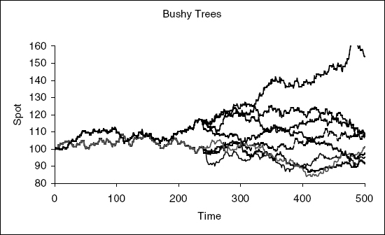
FIGURE 10.1 Broadie and Glasserman method. We simulate P paths up to the first exercise date, then divide each path into P new paths. At the second exercise date, we divide each of the P² paths into P new paths, and so on up until the maturity of the option.

We can now go back to the penultimate early-exercise date, T_N−2; again, we discretize the state-space and start a Monte Carlo simulation at each point, simulating P paths from T_N−2 to T_N−1. For each path, we can decide whether the option would be exercised at T_N−1 based on the exercise value at T_N−1 and the expected continuation value there, which we estimate by interpolating between the points at which we started our first set of Monte Carlo simulations. For each new set of paths, we average over the paths to calculate the expected continuation value at time T_N−2 as a function of the discretized state-space there. This is shown in figure 10.2.

We can iterate this until we get back to the evaluation date. This approach scales much more nicely with the number of early exercise dates and paths than the Broadie and Glasserman approach. However, it is still prohibitively slow, especially when we have to discretize in several dimensions at each fixing date. The time taken using P paths per starting point and M restart points per fixing in each of d directions is proportional to M^dP. Assuming the expected continuation value is a smooth function and we interpolate linearly, we will have a discretization error that scales as 1/M². To get convergence in our price, as we would expect from Monte Carlo, we therefore need M α P^1/4, making the CPU time scale as P^1+d/4.

In high-dimensional problems, this scaling can make the method completely impractical. No method based on calculating the expected continuation value at a discrete set of points across state space will be able to cope with very-high-dimensional problems as there is too much information to store or calculate. Take the example of an option on a basket of 20 stocks. If we try to estimate the expected continuation values on an M²⁰ point mesh, even with M = 3, that is 3.5 × 10⁹ values to store.

FIGURE 10.2 Regularly spaced restarts. At each early exercise date, we discretize the state space and for each point we simulate P paths up to the following exercise date and average to get the expected continuation value.

10.4 THE LONGSTAFF AND SCHWARTZ ALGORITHM

The Longstaff and Schwartz algorithm [189] is an algorithm for combining backwards induction and Monte Carlo simulation that overcomes the scaling of the previous two methods at the expense of introducing some bias into the answer. The algorithm is sometimes called least-squares American Monte Carlo.

As with the previous methods, we try to use Monte Carlo simulation to find the expected continuation value (CV^e) for each path at each early exercise date. As discussed in the previous section, we cannot hope to find CV^e as a function of all the Markov factors in a high-dimensional problem. In least-squares Monte Carlo, we instead try to reduce it to a function of a few relevant quantities: the regression variables. If we choose the regression variables well, this will drastically reduce the dimensionality of the problem of calculating CV^e. However, if we do not choose good regression variables, we will throw away useful information and find a bad exercise strategy and hence a biased price.

10.4.1 The Algorithm

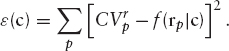
The strategy is as follows. We simulate P complete paths up to the maturity of the option, then work backwards through the exercise dates. Assuming we have not exercised the option early, we calculate all of the payments made after the last early exercise date (T_N−1) and discount them to that date (for each path). We refer to this value as the realized continuation value, for each path p just after the early exercise date. For each path, we also calculate the values of some regression variables (observable at T_N−1), on which we think the estimated continuation value will depend strongly. We then let the estimated continuation value, CV^e(T_N−1), be some parameterized functional form of the regression variables and try to find the parameters that gives the best fit (in a least-squares-error sense) to the realized continuation values. If our CV^e function has parameters c^N−1, we can write

We try to find the parameters c^N−1 that minimize

Now that we have the function CV^e, we have an estimate of the expected continuation value for each path. We can use this to decide whether the option would be exercised for each path by comparing with the exercise value for the path at that exercise date: EV_p. If the holder of the option has the right to exercise, it will be exercised if , whereas if the issuer has the right it will be exercised if . According to this strategy, the realized continuation value for path p just before the exercise decision is made, is EV_p if we exercise and if we do not.

Note that although we use to determine whether or not we exercise, the value we get if we choose not to is . This differs from the approach in the previous section where we set the realized value to (because was not available). This approach matches what would happen in real life and gives rise to a less biased result, as will be explained later.

Having calculated the realized continuation value just before the exercise date T_N−1, we discount these values back to date T_N−2 where they become We repeat the above procedure to calculate and so and so on. We iterate this until we reach the evaluation date and have parameterized expected continuation values, CV^e, for each of the early exercise dates.

We could average over the realized continuation values for each path at the evaluation date to give the price of the option. However, this gives rise to a slight bias (the foresight bias) as the exercise decision for each path will weakly depend on the realized continuation value for that path, through the regression coefficients. We discuss this bias in more detail in section 10.5. It is common practice to remove this bias by using a separate set of Monte Carlo paths to price the option.² We will refer to the two sets of paths as the regression paths and the pricing paths.

With each of the pricing paths, we can repeat the above backwards-induction algorithm (but omitting the regression step and using the previously calculated regression coefficients) to find Alternatively, we can loop forward over the exercise dates until we find the date at which the option will be exercised; we then discount the exercise value at this date to the evaluation date to give

10.4.2 Example: A Call Option with Monthly Bermudan Exercise

To demonstrate the regression phase of the algorithm we will consider the simple example of a Bermudan option with monthly exercise dates and a maturity of two years. The strike of the option is set to 100, which is the current spot price.

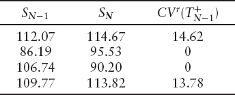
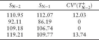
If we price this with deterministic volatility, hazard, and interest rates, then the estimated continuation value at time T_N−1 can only depend on the stock price at that time, so we choose this as our regression variable. The first two columns of the table below show the values of the stock at times T_N−1 and T_N. If we choose not to exercise the option at T_N−1, we will eventually receive max (S_N − 100, 0) at T_N. Discounting this back to T_N−1 (using the discount factor of 0.997) gives the realized continuation values shown in the third column.

Our decision on whether or not to exercise will be based on the estimated continuation value, which we will model as a cubic function of the regression variable (S_N−1):

Taking all the paths into account, we try to find the regression coefficients, a, b, c and d, that minimize equation (10.4). (Details of how to do this are given in section 10.5.2.) We find the least-square error comes from the polynomial

Figure 10.3 shows the results of fitting a cubic function to 2000 paths. The points are the realized continuation values, and the line is the above cubic function.

The table below shows the same four paths but we have added two extra columns. The fourth column shows the estimated continuation value found using equation (10.5), and the fifth column shows the value we get if we choose to exercise immediately.

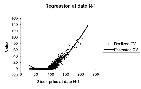
FIGURE 10.3 Result of fitting a cubic to the realized continuation values at the penultimate exercise date of a Bermudan call option.

For the first path, CV^e < EV, so we choose to exercise the option immediately. For the remaining three paths, CV^e > EV, so we choose not to exercise the option. The final column of the table shows the realized continuation value for each path just before the exercise decision. Note that for the third path, we decide not to exercise but the option ultimately expires worthless; not exercising was the best decision we could make with the information available at the exercise date.

For the next step in the regression phase, we take the realized values at date T_N−1 and discount them back to date T_N−2 where they become the realized continuation values, CV^r. The discount factor for T_N−2 to T_N−1 is 0.997, giving the following results.

We have included S_N−1 only for comparison with earlier tables; it is not used in this step of the regression phase. Now we have a new set of regression variables (S_N−2) and corresponding realized continuation values, CV^r, so we repeat the above step to estimate CV^e at date T_N−2. We repeat this until we get back to the evaluation date.

10.5 ACCURACY AND BIAS

In the above algorithm, we have four main sources of error—three in the regression phase and one in the pricing phase.

Like any Monte Carlo price, both the regression and pricing phases suffer from random errors. If we use too few paths in the pricing phase, our result will not be very accurate. Similarly, if we use too few paths in the regression phase, the regression coefficients will not be very accurate, which in turn means our exercise strategy will not be optimal.

For options with a single regression variable, such as the one considered above, the error coming from the pricing phase is likely to be much bigger than the error coming from the regression phase, for the same number of paths. The only points where the accuracy of the regression coefficients matter are the points where CV^e and EV cross over and we move from a region where it is optimal to exercise to a region where it is optimal to hold on to the option—in other words, the exercise boundary.

If our function CV^e is slightly wrong, the position of the exercise boundaries (and therefore our exercise strategy) will also be slightly wrong. However, in the vicinity of the true exercise boundary, it makes little difference whether we exercise or hold on to the option as both choices result in very similar prices. Small errors in CV^e therefore have a much smaller effect on the overall pricing—in fact the error in the pricing scales as the square of the error in the exercise boundary.

A more important source of error comes from the fact we are modeling CV^e by some smooth parameterized function. This might not have enough freedom accurately to approximate the true expected continuation values. In figure 10.4, we show CV^e for the penultimate exercise date of the Bermudan call approximated with cubic and quintic functions, as well as the exact answer.

Clearly the cubic and quintic do not—indeed cannot—fit the real expected CV for all spots, although the quintic does a much better job than the cubic. These errors do not go away as we increase the number of paths used in the regression phase, which means that for this option, American Monte Carlo gives only a lower bound to the price. This is a general result: The Longstaff and Schwartz algorithm always gives a suboptimal exercise strategy and so if the holder has the right to exercise, the algorithm will always give a lower bound, whereas if only the issuer has the right to exercise, the algorithm will give an upper bound to the price.

Figure 10.4 also demonstrates why we use CV^r and not CV^e as the realized value of the option if we choose not to exercise. The inaccurate values of CV^e have only a small effect on the pricing when we use them only to determine the exercise strategy; were we to use them as the realized values for nonexercised paths, the errors in CV^e would become errors in our final price, potentially leading to very biased results. We would also have no guarantee that we had found a lower (or upper) bound to the price.

The polynomials in figure 10.4 do not agree closely with the more accurate piecewise-linear function. We show how to improve on this in section 10.5.1.

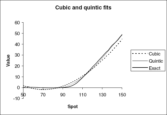
FIGURE 10.4 Fits to the expected continuation value at the penultimate exercise date of a Bermudan call option.

The final source of error is the foresight bias mentioned in section 10.4.1. In the regression phase, the exercise decision for each path depends on the regression coefficients, which in turn depend on the realized continuation value for that path. We therefore have a small foresight bias; for a low number of paths, our exercise strategy will be better (for those paths) than the real-world exercise strategy. In figure 10.5, we show the results of pricing an at-the-money call option, exercisable after 2y and 4y.

Generally, this foresight bias will be much smaller than the random error in the price, and can be reduced by using independent pricing and regression paths. However, for derivatives with many early exercise dates, this error may be compounded up until it is significant. See Fries [190] for more details.

10.5.1 Extension: Regressing on In-the-Money Paths

In the above example with the cubic function, CV^e becomes slightly negative for some out-of-the-money paths of the stock price when in reality we know it must be slightly positive. This is just an artifact of fitting a polynomial to the data. In the region where CV^e becomes negative, our strategy would tell us to exercise the option even though we receive nothing and give up the chance to receive a positive amount at the next exercise date. In reality, we would never consider exercising the option unless it were in-the-money. We can use this to improve our pricing.

Since we will consider exercising the option only when it is in-the-money, we also only need to know CV^e for the paths where the option is in-the-money. Instead of fitting a cubic to all the points in figure 10.3, we can just fit it to the in-the-money points (i.e., where the stock is above the strike at T_N−1). The result of doing this is shown in figure 10.6.

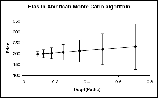
FIGURE 10.5 Foresight bias when pricing an in-the-money call, exercisable after 2y and 4y. The line shows the average price of the option from 10,000 independent pricings, each using P paths, against P^−0.5. The error bars are one standard deviation of the random errors in each individual pricing. Here the bias scales as P^−0.5, and is equivalent to approximately one third of a standard deviation.

FIGURE 10.6 Cubic and quintic fits to the expected continuation value using only the in-the-money paths.

The fit to the in-the-money region is now much better than when we tried to fit all points at once. The fit to the region that's out-of-the-money is truly abysmal, but since we know we're not going to exercise there anyway, it doesn't matter.

For any option where we know we will not exercise if some condition does not hold, we can improve the performance of the algorithm by only regressing on paths that could potentially be exercised, and never exercising paths that can never be exercised (regardless of the estimated expected continuation value).

10.5.2 Linear Regression

We will now go into more detail on how to fit the CV^e functions.

Assuming we have a set of regression variables r_p and realized continuation values , how should we fit a function CV^e(r_p)? Dropping the N − 1 indices from equation (10.4), we want to minimize

For a general nonlinear function of the coefficients, we would have to use some general minimization algorithm like the Newton-Raphson algorithm described in section 3.6.1. However, since we may have thousands or even millions of paths, this will be incredibly slow. For this reason, we restrict the allowed functions to linear functions of the coefficients. We write

Letting

we have

where

R is the vector

and M is the symmetric matrix

Note that once we have computed A, R, and M, the computational time taken to calculate the mean-square error ε for a given trial set of parameters, c, is independent of the number of paths. This makes linear regression much faster than fitting some nonlinear function.

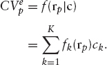
Differentiating equation (10.6) with respect to c_k gives

To find the coefficients that minimize ε, we need to solve the simultaneous equations

Since M is a symmetric matrix, we can invert equation (10.7) by finding the Cholesky decomposition of M. However, it is possible that one or more of the regression coefficients has no effect on the solution or that some of the functions are linearly dependent, either through the choice of regression functions or through using an insufficient number of paths. There is also the possibility that if the real matrix M is close to singular, then numerical rounding/truncation errors may cause it to have negative eigenvalues and so according to equation (10.6) there will be no minimum of ε. Cholesky decomposition will fail if M has zero or negative eigenvalues, so instead we use singular value decomposition as a more robust way of solving equation (10.7).

In singular value decomposition (SVD), we decompose the matrix M as

where U and V are orthogonal matrices and D is a diagonal matrix containing the singular values of M (i.e., the eigenvalues of M²). Since M is a real, symmetric K × K matrix, U, V and D are also K × K matrices and we have

Now if there exist any linear combinations of the regression coefficients that are zero for all paths (i.e., the regression functions are not linearly independent), there will be elements of D that are zero. The corresponding columns of V are called the nullspace of M. If the vector e is in the nullspace, we have Me = 0, and so any component of c in this direction has no effect on ε and so cannot be determined. We can therefore set the components of c in these directions to something arbitrary without affecting the result. To set the components to zero, we set the corresponding elements of D⁻¹ to zero.

In fact, very small singular values may be the result of numerical rounding errors and so it is best to ignore all singular values below some threshold. Numerical Recipes [70] suggests ignoring all singular values which are less than ∈ of the largest singular value, where ∈ is machine precision (about 10⁻¹⁵ for double-precision numbers) by setting the corresponding elements of D⁻¹ to zero.

10.5.3 Other Regression Schemes

If the expected continuation value we are trying to approximate is not a particularly smooth function of the regression variables, fitting it with a polynomial will smooth out features that we want to capture. A common alternative is to break the phase space up into smaller regions and fit either a constant or some other functional form in each region. If we split the domain of possible regression variables into groups A_i, we can write the expected continuation value as

One way of doing this is to perform a separate regression for each set of paths, the i'th set of paths being all the paths for which r_p ∈ A_i. The limit of fitting just a constant for each group is Tilley's method [191].

An alternative method is just to treat

as separate regression functions and do a single regression but with many regression functions. The SVD method described in section 10.5.2 is robust enough to handle this. The “exact” lines in figures 10.4 and 10.6 were produced by fitting piecewise-linear functions in this way.

The drawback of this approach is that the more partitions are used, the fewer paths fall into each partition, so we must use a greater number of overall paths to guarantee a good accuracy of the estimated continuation value. We must also be careful how we choose the partitions, making sure that we are likely to get a reasonable number of paths in each. This approach can work well for low-dimensional problems where the phase space can easily be partitioned, but for higher-dimensional problems, the number of partitions (and consequently the number of paths we need to use) may make the algorithm too slow.

10.5.4 Upper Bounds

The Longstaff and Schwartz algorithm gives a lower bound for options where the holder has the right to exercise. Upper bounds to the price can be found using strategies proposed by Rogers [192] and Andersen and Broadie [193]. The value of an option can be expressed as

where τ is a stopping time and h_t is the value of exercising at time t. In other words the option is worth the expectation of the discounted cashflows from the optimal exercise strategy. The Longstaff and Schwartz algorithm effectively tried to find the optimal stopping strategy, but in reality would always find a less-than-optimal strategy and hence give a lower bound to the price.

In Rogers and the like, they express the price in terms of a dual formulation

where M is some martingale. The strategy then becomes to find the M that minimizes the above expression. The better the choice of M, the tighter the upper bound.

10.6 PARAMETERIZING THE EXERCISE BOUNDARY

In the previous section, we discussed the Longstaff and Schwartz algorithm, where the expected continuation value is parameterized as a function of some regression variables. The estimate of the expected continuation value was only used to decide the exercise strategy; all that mattered was whether it was greater or less than EV.

This gives rise to an alternative strategy suggested by Andersen [194]. Instead of parameterizing the expected continuation value, we can parameterize the exercise boundary itself. This strategy can only work if we already have some knowledge of the topology of the exercise regions (e.g., how many exercise boundaries we need to find). If we allow the strategy to find an arbitrary number of exercise regions, we will end up with an exercise region around each path where CV^r < EV (i.e., perfect foresight).

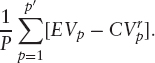
As an example, consider the example of the Bermudan call option again. We know that we only exercise such an option before maturity in order to receive a dividend. We give up some optionality in exercising the option, but the value of this optionality decreases the more in the money the option becomes, so there is some stock price above which we will exercise the option and below which we will not. We can find the best exercise boundary for a set of paths by finding the path p′ that minimizes

If we sort the paths by their stock prices, we just need to find S_p′ that minimizes

As we increase the total number of paths used, S_p′ will converge to the correct exercise boundary. Note that this strategy is biased—the exercise strategy will always be better for those paths than we could hope for in real life, so this procedure will give an upper bound to the price. If we then price the option with a new set of paths but using the same exercise boundary, we can generate a lower bound to the price.