CHAPTER 6

Credit Modeling

6.1 INTRODUCTION

The growth witnessed in the credit derivatives market in recent years has led to the introduction of equity hybrid structures that depend on the creditworthiness and the performance of an equity underlying. Convertible bonds constituted the first generation of these structures and are still the most liquid of them, while the equity default swap remains the main innovation in this field.

This chapter presents a methodology to value derivative securities written on equity underlyings subject to credit risk. Arbitrage-free valuation techniques are employed, and the methodology is applied to derivative securities written on assets subject to default risk as well as to pure credit derivative instruments.

6.2 BACKGROUND ON CREDIT MODELING

The risk of default is the financial loss that a counterparty would bear if a reference entity does not honor its commitments. This is in general called a credit event and could range from downgrades by a rating agency to failure to pay debt to complete liquidation. In theory, every financial transaction embeds this kind of risk regardless of the counterparties involved. Estimating the likelihood of occurrence of a credit event is the center of any methodology aiming at modeling credit risk or default risk. However, this is not sufficient for the pricing of contingent claims sensitive to default risk. Indeed, we need to model the loss given default (or recovery), risk-free interest rates, and in the case of multiname securities, the dependency between the credit events.

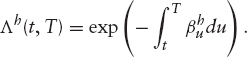
There are two main routes to modeling default risk, the structural approach and the reduced-form or intensity, based approach. In the first approach, we make explicit assumptions about the capital structure of the company, its debt, and the dynamics of its assets. In the reduced-form approach, the dynamics of the default are exogenously given by a default rate (intensity). Intensity-based models focus directly on describing the conditional probability of default without the definition of the exact default event. The use of a Poisson process framework to describe default captures the idea that the timing of a default takes the investor by surprise. Technically speaking, either the default time τ is a stopping time in the asset filtration (structural models) or it is a stopping time in a larger filtration (intensity models).

6.2.1 Structural Approach

The firm value model was introduced by Black and Scholes in 1973 and Merton in 1974. It consists of defining the default time as the time τ that the underlying process, the assets of the firm, hits a certain barrier.

Standard Approach Consider a company with market value V_t at time t, which represents the expected discounted value of its future cash flows. The company has a debt modeled as a zero-coupon bond with face value D and maturity T. If the company cannot honor its commitments at maturity, the debtors take control of the company.

The firm value V_t (also called asset price) is modeled as geometric Brownian motion and its dynamics are given as follows:

The default event is defined as the inability of the company to pay its debt at maturity; that is, V_T < D. The default probability is therefore given by

where is the leverage ratio.

The bondholder receives at maturity D(T, T) = min(V_T, D), which could be written as

Therefore, the bondholder is long a default-free bond with a face value D and short a put option on the assets of the company.

On the other hand, the equity value E_T = max(V_T − D, 0) is a call option on the assets of the company. The values today of the debt and equity of the company are given by

where B(0, T) is the default-free zero-coupon bond.

The credit spread is defined as the excess return, above the risk-free rate, demanded by investors for bearing the default risk of the underlying entity. Its expression, using the formulas above, is given by

First-Passage Approach In the standard approach, the value of the company can reach any value between today and the maturity without triggering the default event (value of the company at any point in time before maturity can be below the face value of the debt). The test for default or no default is done only at maturity. The first-passage approach, on the other hand, defines the default event as the first time the value of the company drops below a predefined barrier H.

Given the dynamics (6.1), the probability of default is given as follows:

Within this approach the bondholder receives at maturity

The bondholder is therefore long a default free zero coupon bond with face value D, a down-and-in call on the assets of the company, and short a put on the assets of the company.

On the other hand, the equity value at maturity is given as follows:

that is, the equityholder is long a down and out call on the assets of the company. The values D(0, T) and E₀ of the debt and equity today are given by

where and D(0, T)^standard are the values of the equity and debt at time 0 given in the standard approach described above.

The derivation of these formulas could be found in [130].

The credit spread is therefore expressed as follows:

Discussion The calibration of structural models is problematic, as the value of the firm is not directly observable in the market. The face value and the maturity of the debt is not easy to estimate from the balance sheet given the complexity of the capital structure of the company. Indeed, we often have a mixture of short-, medium-, and long-term debts as well as different seniorities. The barrier level, in the case of a first-passage approach, is another parameter that is not easy to estimate, and its definition is generally ad hoc and conditions the occurrence of default event.

Another drawback of the two approaches described above is the fact that the default cannot happen immediately. This has been addressed by random barrier models such as credit grades. However, this adds even more complexity in terms of the calibration as we need to calibrate the volatility of the barrier level in addition to all other parameters.

Nevertheless, this approach could be useful to provide predictive tools related to upcoming default events. Indeed, a pre-default event could be defined as the first time the asset value is below a certain level higher than, but close to, the default barrier, and users of structural models observe the evolution of the so-called “distance-to-default” or the marginal default probabilities. From a mathematical point of view, this means that the default time τ is predictable, a stopping time with respect to the asset filtration. Unfortunately, market reality is different, as we do witness spread movements as well as jumps to default that happen in a surprising way.

The inability of structural models to properly describe the default event is a drawback well described by Madan in “Pricing the Risks of Default” (2000):

6.2.2 Reduced-Form Approach

In reduced-form or intensity-based models, the dynamics of the default are described exogenously and directly under the pricing measure. We model the instantaneous likelihood of default through the hazard-rate process.

Definition of the Hazard Rate of a Default Time

Hazard rate: Deterministic case Let us consider a security with default time τ. τ is a continuous random variable measuring the length of time from today to the default time.

Let F(t) denote the distribution function of τ:

We also define the survival function S(t) by

As to the probability density function, it is given by

The distribution of the random variable default time can be specified with the hazard-rate function, which gives the instantaneous default probability for a security that has attained time x, given survival to this time:

The function

used in statistics under the name of hazard-rate function, is the conditional probability density function of τ at time x, given survival to that time.

The hazard-rate function can easily be linked to the survival function as follows

We get

In the same way,

Lastly, distribution and density functions of the default time τ can be expressed as a function of the hazard rate function as follows:

These relationships show that modeling a default process is equivalent to modeling a hazard-rate function.

Hazard rate: General case Let us define the default process by N_t = 1_τ≤t, where τ is the default time. It is assumed that the increasing one-jump process N_t admits an absolutely continuous compensator Δ_t, where Δ_t is a predictable and increasing process such that N_t − Δ_t is a martingale [131]:

where the non-negative predictable process h stands for the intensity process or hazard rate. With a constant intensity h, for example, default is a Poisson process with intensity h. More generally, for t < τ, h_t can be viewed as the conditional rate of arrival of default at time t, given all information available up to that time. Roughly speaking, for a small time interval of length Δt, the conditional probability that default occurs between t and t + Δt, given survival to t, is given by h_tΔt.

We consider two increasing and complete information filtrations such that

the default time τ being outside the span of F = F_T.

Now, the process

is a martingale.

The following result will allow us to eliminate the jump process N_t from the evaluation of any derivative payoff.

LEMMA 6.2.1 We admit the following result:

Let us define S(t, T) the probability of no default (or survival probability). It can be expressed as

A direct application of Bayes's theorem gives

where the last equality directly follows from (6.10).

This important result generalizes the results of the previous section, allowing now the hazard-rate function to be stochastic.

Construction of a Default Time In this section, we give a background on how to construct a default time.

Let be a filtered probability space, and Z_t a diffusion process on this space. Let θ be an exponential random variable with intensity 1 independent from Z_t.

We define the default time τ as the first time when the process is above the random variable θ:

where h is a positive function. An equivalent way of defining τ is

where N_t is a Poisson process with intensity 1 independent of F = σ(Z_t, t ≥ 0).

Therefore, the conditional distribution of the default time τ given F_t(F_t = σ(Z_s, t ≥ s)) is given by

We introduce the filtration the enlarged filtration with respect to which τ is a stopping time. Indeed, τ is not stopping time with respect to the filtration¹ F_t; otherwise, we would have and not (6.12).

For the pricing of contingent claims on defaultable securities, the following theorem is essential:

THEOREM 6.2.1 Let X be an integrable random variable; we have the following result:

where

Modeling a hazard-rate function provides us information on the immediate default risk of each entity known to be alive at a given time t and facilitates comparisons with other entities. Also, as we will see, this kind of modeling can be easily adapted to the stochastic default case. Linked to this point, the strong similarities between the hazard-rate function and the short rate allow us to borrow some modeling techniques from the short-rate world.

6.3 MODELING EQUITY CREDIT HYBRIDS

We are given a filtered probability space where all processes are assumed to be defined and adapted to the filtration We will be working in an arbitrage-free setting, and we will be considering the dynamics of the involved processes directly under the risk-neutral measure .

6.3.1 Dynamics of the Hazard Rate

We will exploit the results of the previous sections to choose a stochastic diffusion for the hazard-rate process. The similarities between the hazard rate and the short rate legitimate the use of some modeling techniques proper to the short rate. Two kind of diffusion could be employed to model the dynamics of the hazard rate: affine diffusions and mixed diffusions.

Affine Diffusion Models The tractability of affine diffusion models [132] makes them prime candidates for the modeling of the hazard rate process. Indeed, we can easily obtain closed-form solutions for the survival (default) probabilities in some cases, and we only need to solve an ordinary differential equation in some other cases.

An affine diffusion model is given by the following stochastic differential equation:

where μ and σ² are affine functions of h_t; that is, μ(t, h_t) = a₁(t) + b₁ (t)h_t and σ²(t, h_t) = a₂(t) + b₂ (t)h_t. The survival probability (the equivalent of a zero-coupon bond) is given by

where m(T) and n(T) are deterministic functions of T, a₁, a₂, b₁, and b₂.

Note that the affine diffusions models remain tractable and yield similar expression for the survival probabilities in the multidimensional case.

Mixed Diffusion Models This class of models contains the CEV kind diffusion given by

These models have the drawback of being computationally unattractive (except for γ = 0 or γ = 0.5, because we end up with an affine diffusion).

The model choices we make in the remainder of this chapter are based on affine models. Precisely, the dynamics we will study for the hazard-rate function are the Hull-White diffusion in the first stage. An extension to include jumps is studied later.

6.3.2 Model Choice

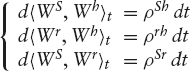
Assuming Hull-White-type diffusions for the hazard rate and short rate, we end with the following system of SDEs:

with

where N_t = 1_τ≤t, with τ being the inaccessible default time. N_t is taken to be independent of all the Brownian motions, W^S, W^h, and W^r. y_t = μ_t + δ_t, where μ_t and δ_t are the dividend yield and repo rate, respectively.

Initially, and in order to allow for a more tractable model, instantaneous short rate is taken to be deterministic. The extension to stochastic interest rates is straightforward and will be discussed later.

Study of the Hazard Rate Dynamics As specified above, the dynamics of the hazard rate are given by

The solution to (6.14) is given by

We have

with

This is true for all affine-type diffusions as mentioned earlier, that is, for all diffusions for which the drift term and the square of volatility are linear functions of h_t

Furthermore, the survival probability S(t, T) satisfies the PDE below:

with the terminal condition

Replacing the expression of the survival probability (6.15) in the PDE, we obtain

where m_t(t, T) and n_t(t, T) are the first derivatives of m(t, T) and n(t, T) with respect to t.

By separating terms that do not depend on h_t and those that do depend on h_t, we get a polynomial of degree one with respect to the variable h_t; both coefficients will be equal to zero. We therefore have the following system of differential equations:

and

Integrating these equations, we get

Let us define the T-maturity instantaneous forward hazard rate by

with

We have

where

and

where

Thus,

This expression can be rewritten as

with

such that

Consequently,

and

Finally, the parameter θ^h is uniquely determined and given by

However, in practice, we do not need to calibrate as it is implied by today's credit curve. The above result has only a theoretical interest in showing that is uniquely specified. Note also that the expression of the survival probability could be derived by simply computing the expectation which is easy given that exp is a log normal variable.

Dynamics of the Survival Probability The expression of the survival probability under the risk-neutral measure is given by

Given this expression, we show that its dynamics under is given by

where

with

Furthermore, we have that

This is going to be very useful when pricing various derivatives as we discount with exp The above results are very similar to the ones obtained in the case of short-rate models.

6.4 PRICING

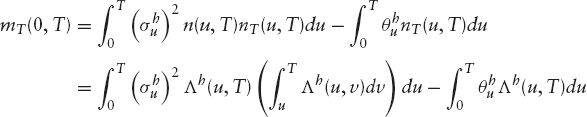
6.4.1 Credit Default Swap

credit default swap (CDS) is a financial agreement between two counterparties in which the protection buyer makes regular fixed payments during its term, whereas the protection seller is binded to making a payment upon the default of a reference entity. The default event definition could range from the failure of making a simple interest payment to complete bankruptcy. The default payment could be made at maturity (standard or European type) or at time of default (American type).

The CDS price (spread) is the premium value that makes the agreement a fair contract, that is, the default leg is equal to the premium leg. As mentioned above, we assume that the interest rates are deterministic (independence between the default process and the interest rates yield exactly the same results), and the default payment is made at the time of default (American case).

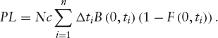
Premium Leg The premium leg is the price of a risky coupon bond with notional equal to the one of the CDSs and where all the payments are discounted using risky zero rates (default-free zero bond times the survival probability). Let (t₁, t₂, …, t_n = T) be the set of payment dates where T is the maturity of the CDS, N is the notional of the swap, and R is the recovery rate of the reference entity assumed to be constant.

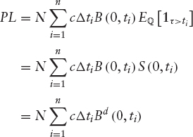
where Δt_i is the day count fraction for the period [t_i−1, t_i], t₀ = 0 and B^d (0, t_i) is the risky zero coupon bond defined as follows:

Note that this expression is not true if we have correlated hazard rate and short-rate processes.

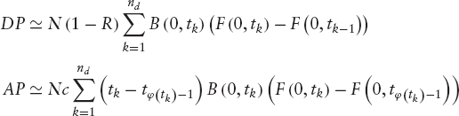
Default Leg The default leg is the expected value of the default payment (DP) minus the accrual premium payment (AP). These two quantities are computed as follows:

where f(0, T) is the instantaneous forward rate given by: and

The spread of the credit default swap is the value of c that makes the default leg equal to the premium leg, hence:

Note that credit default swaps are quoted in spread in the marketplace.

6.4.2 Credit Default Swaption

Let's call CDS_{S, N}(t), the value at time t of a CDS contract starting at time T_S and maturing at time T_N, with notional N and recovery rate R.

Similar to a CDS starting today (6.21), the expression of CDS_{S, N}(t) is given as follows:

where

• S(t, u) is the survival probability from t to u conditional to no default at time t.
• Δt_i is the length of time expressed in fraction of years between T_i−1 and T_i.
• B(t, u) (B^d(t, u)) is the default-free (risky or defaultable) discount factor from t to time u.
• c is the premium paid at every payment date by the protection buyer.

The CDS par spread s_N is defined as the rate c that cancels the present value of the swap, and is given as follows:

CDS Option Price Let's call C_{S, N}(t) ≡ C_{S, N}(t, T_S, K) the value at time t of a call option maturing at time T_S and struck at K written on the CDS spread contract CDS_{S, N}(t).

If the default occurs before the option maturity T_S, two different treatments are possible: either the option is knocked out and its value drops to zero or the option remains valid and pays the default protection at maturity.

We focus here on the pricing of the knock-out CDS whose price at time T_S is given by

where B^d (t, T) is given by (6.20).

The payoff of the option can be rewritten as

Let us define the level of the swap at time t, LVL_{S, N}(t) as

Writing the expression of the call price under Q^LVL, we get

Under the CDS spread, s_N, is a martingale. Its diffusion is assumed to be log normal and can be written as

The CDS option price is therefore given by the Black formula as follows:

where d₁ and d₂ are given by

Link between CDS Spread Volatility and Hazard Rate Volatility The objective of this section is to express the CDS spread volatility as a function of the hazard rate volatility For the ease of the computations we set N = 1.

At time t, the CDS spread, s_N(t), is defined as

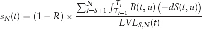
where LVL_{S, N}(t) is given by (6.22).

Recall the diffusions of the survival probability S(t, T) and the instantaneous forward hazard rate fh(t, T) under the risk-neutral measure :

and

where σ^SP(t, T) and σ^fh(t, T) are given by

Applying Ito to the process s_N(t), we get

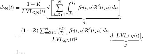
where the remaining terms are drift related.

The expansion of the terms A and B gives

We can now relate the CDS spread volatility to the hazard rate volatility through σ^fh(t, u) and σ^SP(t, u), as follows:

6.4.3 European Call

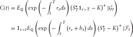
Deterministic Interest Rates Case At a given time t, the price of a standard call option struck at K and maturing at T is given by

where is the nondefaultable stock and its diffusion is given as follows:

and we have

On the other hand, B(t, T) is the nondefaultable zero-coupon bond of maturity T. After some calculations, we obtain

where is the T-forward value of the asset.

The expressions of d₁, d₂ and are given by

Stochastic Interest Rates Case Under the risk-neutral measure, the dynamics of the asset S_t, the survival probability S(t, T) and the nondefaultable zero-coupon bond B(t, T) are respectively given by

where r_t is the instantaneous short rate and

As for the survival probability, the diffusion parameter of the zero-coupon bond is defined as

where

N_t being independent of the rest of the random terms (Brownian motions), we will focus on the nondefaultable stock. The price of a European call option is given as follows:

The expressions of d₁, d₂ and are given by

where

Case Studied To minimize the number of parameters to estimate, we chose to work within a deterministic interest rate framework. As shown above, the extension to a stochastic interest rate framework is straightforward, but requires some estimation of the correlation between the short rate and the hazard rate.

In the next section, we are going to focus on the calibration of the model's parameters exploiting the above results on the pricing of some derivatives products within the modeling framework.

6.5 CALIBRATION

6.5.1 Stripping of Hazard Rate

Calibration of Default Probabilities Credit default swaps are the most liquid credit derivative instruments on a reference entity; therefore, we can use them to back out default probabilities. This is done by discretizing the integrals in the CDS price formula given by (6.21). Indeed, we can write the default and accrual payments as follows:

where n_d is the number of discretization dates, φ(t_k) is the next coupon date after t_k, and is the default probability. The premium leg, on the other hand, as a function of default probabilities, is equal to

By bootstrapping we can we get back the default probabilities F(0, t_k), k = 1, …, n_d.

Hazard Rate Curve Estimation The hazard function is assumed to be a piecewise constant function, between the maturity dates of the credit default swaps on the reference entity, and is given as follows:

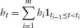
The default probability is therefore given as follows:

where as before φ(t) is the next date (in the sequence t₁, t₂, … t_m) after t, and i^* is the corresponding index (i^* ∈ {1, …,m}). The hazard rate h_i is then given by

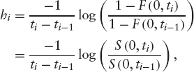
where S(0, t_i) is the survival probability up to date t_i.

6.5.2 Calibration of the Hazard Rate Process

As discussed above, we can back out the default probabilities and hazard rate curve seen from today using credit default swaps. Similarly to interest rate models (see chapter 3), the function does not need to be calibrated and is fully determined by today's survival (default) probabilities. Therefore, we only need to calibrate the volatility and mean reversion parameters and which we can do using the credit default swaption prices and the relationship given in (6.25).

Recall the relationship between the CDS option implied volatility and the CDS spread local volatility given by the following expression:

The main assumption relies on the log-normal distribution of the CDS spread under its natural measure. Therefore, we can rewrite (6.25) such that we can have an explicit dependency between and by replacing σ^fh and σ^SP by the expressions given in (6.24) and (6.23). We can therefore use a least square minimization to compute a piecewise constant and .

6.5.3 Calibration of the Equity Volatility

The calibration of the equity diffusion consists of the calibration of the local volatility parameter σ^S to standard market option prices. To this end, we will use the formula (6.26) derived before for the price of a European call option in the framework where the stock jumps to zero as the default event happens.

Given that equity option prices are more liquid than their CDS counterpart, we will use the former to calibrate and ρ^Sh simultaneously.

6.5.4 Discussion

For most names, and due to the lack of liquid credit default swaptions available on the credit market, the parameters β^h and σ^h could be calibrated bond options. If none of these is liquid enough, calibration to historical data is sometimes done and the adjustment of these parameters (historical vs. risk-neutral) is left to the discretion of the trader.

Sending β^h to 0⁺ in (6.14), we get a Ho-Lee kind diffusion for the hazard rate such that the mean reversion effect disappears. This property may prove to be useful when dealing with a credit quality with no particular mean-reverting behavior or with historical data too limited to be used to assess a value for this parameter.

The introduction of defaultable bonds written on the same credit name into the set of calibration instruments could allow us to calibrate the hazard-rate parameters to the market. Note that the presence of these instruments in the hedging strategy legitimates their use in the calibration. Furthermore, despite their close link to the CDS product, their difference in liquidity reflects the different nature of the risk they bear. Convertible bonds, provided some liquidity, could also be added as calibration instruments.

In the following section, we are going to present an extension to this framework by introducing jumps in the stock diffusion and hazard-rate diffusion. This will enable us to capture correctly the movements of the credit spreads. Indeed, when a downgrade is announced by a rating agency, the spreads widen in a jumpy way.

6.6 INTRODUCTION OF DISCONTINUITIES

A natural extension of the model consists of introducing jump processes within the previous framework to account for the spread-widening effects. The objective is threefold: First, the presence of jumps in the equity process allows us to capture the equity smile that is not explained by the introduction of the credit component. Second, adding some discontinuities to the hazard-rate process will allow us to capture, as said above, the spread movements observed in the market. Last, by describing the jumps in both processes, equity and hazard rate, with the same jump processes, we capture better the joint behavior of the hazard rate and the equity. Indeed, the same jump happens at the same time in both quantities with different amplitudes, which allows to capture the correlation between extreme events.

6.6.1 The New Framework

We model the discontinuities in both processes, equity and hazard rate, with the same Poisson processes and with deterministic intensities and The jump sizes for the equity and for the hazard rate are constant. The reason we introduce two jump processes is to account for downgrades and upgrades where the jump sizes account for the average downgrade and upgrade effects. The three Poisson processes N,N¹ and N² are taken to be independent:

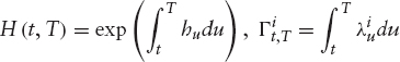
and the hazard rate process is given by

where and are correlated as before with the correlation We set J = 0 such that when the default event occurs, the equity process drops to zero and stays there.

6.6.2 Dynamics of the Survival Probability

We integrate the SDE (6.28) to get the expression of the hazard rate:

For t ≥ s,

Integrating between t, and T, we have:

The survival probability is therefore given by the following expression:

In the above expression, we have made use of the independence between all the random processes involved in the diffusion of the hazard rate (the two Poisson processes and the Brownian motion).

We can also write the expression for exp (the equivalent of the cash bond in interest rate):

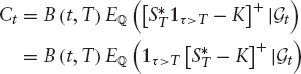
6.6.3 Pricing of European Options

The price of a European call option with a strike K and maturity T is given by

where B(t, T) is the nondefaultable zero-coupon bond maturing at time T.

Therefore,

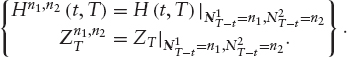
Conditionally to {N_T−t = k}, the jump times (T₁, T₂, …, T_k) have the following law:

Define

and

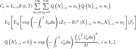
The call price computation requires computing a double summation. Indeed, we have

where the expressions of and are respectively given by

To simplify these expression, we introduce the new quantities:

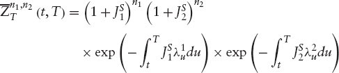
such that

Therefore,

where ₁ and ₂ are given as follows:

We can therefore write the price C_t as follows:

where

It is clear from (6.29) that a direct computation of the price of a European call option is time consuming and a better alternative is needed. In the following section, we apply the Fourier method in order to speed the pricing.

6.6.4 Fourier Pricing

Applying the Carr-Madan technique, we define the dampened call price as follows:

C(t, T, k) is the price of a European option with strike K and maturity T. The Fourier transform of (k) is given by

where is the nondefaultable stock.

with

where ω = iζ + α + 1, and Z^S is independent from W^h such that: The above expression is simplified as follows:

We can therefore compute the call price by inverting the Fourier transform computed above.

This technique is computationally very quick, which is very important for the calibration.

6.7 EQUITY DEFAULT SWAPS

The equity default swap, or EDS, is an instrument whose definition intentionally reflects that of the much-better-known credit default swap (CDS).

The two counterparties to the EDS transaction are the protection buyer and protection seller. The protection that is traded is protection against a stock's reaching a level that is relatively low compared to the reference price (the stock's traded price at the inception of the trade). This level, the barrier, might be 70%, perhaps 50%, or even 30% of the reference price, that is, low compared to barriers typically seen in standard down-barrier options.

The key difference between the EDS and CDS is that the CDS protection is triggered only on a default event, doubtless accompanied by a precipitous drop in the share price of the defaulting company, perhaps to near zero, whereas the EDS protection pays out if the stock drops below a level that is still far from zero, whether or not this is accompanied by a default. (It is perfectly possible for the share price of a company to fall, over a reasonably long period, by a factor of three with no suggestion that the company is close to default nor with necessarily a corresponding fall in its dividend payment.)

This breach of the barrier is known as the knock-in event. We may immediately distinguish two cases: the knock-in event being caused by the stock diffusing across the barrier in the ordinary way (the mechanism by which barriers are breached when barrier options are priced, as they frequently are, in a pure diffusion model such as local volatility); and the event being caused by a default causing the share price to “gap” to below the barrier (perhaps to near zero).

Note that although we distinguish these cases within the context of a diffusion model with jump-to-default, there is no such distinction written into the definition of the structure. Nor, for that matter, is it generally clear from market information what is causing any given move in the stock. An advantage often claimed for EDS over CDS is that the determination of a credit event is less transparent than an observation of a share price, as the latter is based on public market information.

As its name suggests, the EDS is structured as a swap having two legs: the fixed leg and the protection leg, sometimes known as the equity leg. Each leg, of course, is written on the same notional amount N₀. The protection buyer is short the fixed leg: he pays a predetermined coupon stream to the protection seller. This might be x% × N₀ quarterly, for example. The protection seller pays a predetermined amount to the protection buyer in the event of the barrier's being breached. This amount will be y % × N₀ less the accrued on the fixed leg at the time of the knock-in event.

Another variant replaces the fixed coupons with floating, so the payments might be calculated using a LIBOR rate plus a spread. Again, the floating leg payment in the event of a knock-in event is the appropriate accrued amount.

It is possible to extend the equity default swap concept to so-called multiname structures, in which the protection traded, and therefore the definition of the knock-in event, relates to the first of several underlyings to hit its corresponding barrier (compare first-to-default structures in the credit market); all barriers being set at the same level relative to their spot values at the inception of the trade. We will not explicitly describe these here; it is a straightforward generalization. At the time of writing, in the authors' experience, multiname EDSs trade less frequently than single name.

Structuring an EDS EDSs as described above trade in the interbank market. For wider distribution, however, it is common to structure the product as a note.

The buyer pays 100 on entering the position, and receives this amount back from the issuer at maturity unless there has been a knock-in event prior to this. The knock-in event is defined as the first date on which the closing price of the underlying share on the relevant exchange is at or below the barrier. (It is precisely this transparency and simplicity of definition that is the feature argued in favor of the EDS.) The buyer of the note receives a coupon stream, or else it may be a zero-coupon instrument, in which case he receives only a coupon at maturity, in addition to the redemption payment.

In the event of a knock-in, the note is said to accelerate (i.e., terminate early), and the holder receives an early redemption payment much less than 100: only 50, say. He also receives the accrued on the coupon accruing at the time of the knock-in event.

The holder therefore stands to lose a substantial fraction of his investment if the underlying share breaches the barrier. If default were the only process that could trigger this, he would be accepting simple credit risk and would have sold the protection against that risk. Of course, in a model with default and diffusion, either process can cause the knock-in event to trigger. In exchange for accepting this risk, he is compensated with an above-risk-free coupon stream.

This trade can be decomposed into an EDS as defined above, whose protection leg pays 50, plus a bond that knocks out under the same conditions as the knock-in event of the note.

The protection seller (note holder) may also enter into a cancelable swap to mitigate his interest rate risk. Thus, he may agree to exchange his fixed-coupon payment for a sequence of floating payments plus a spread. He would then have interest rate risk only on the spread (the floating payments plus final redemption payment value exactly to 100, irrespective of rates). The cancellation clause would, of course, be precisely the knock-in event of the note.

6.7.1 Modeling Equity Default Swaps

For a general-case multiname EDS priced under stochastic hazard rates, any of the choices for the hazard-rate diffusion given in section 6.3.1 may be realized by brute-force Monte Carlo. There are a number of issues with this:

• Each time step of each path of each underlying requires an interpolation to be made on a local volatility surface, which can be slow. That said, careful implementation techniques can considerably alleviate this problem.
• Structures having many underlyings are computationally intensive to risk manage: for N underlyings, there are obviously N deltas, gammas, and vegas, and off-diagonal gammas. Clearly, this is not limited to multiname EDSs, nor is it specific to Monte Carlo as a numerical technique, but it is a significant issue in modeling and risk managing these positions. Combined with the instability of simple finite difference approximations for the gammas of barrier-type products valued by Monte Carlo, there is a real issue in obtaining this risk for multiname EDS. Exactly the same issue is addressed in section 7.4.1 as applied to another multiunderlying structure type: the Altiplano.
• The simulation requires as parameters the correlations between all pairs of equities and hazard rates. In particular, it requires equity-equity correlations, which we take to be given. It requires also the correlations between equities and their corresponding hazard rates; the calibration of the hazard-rate process provides these. But it also needs correlations between pairs of hazard rates and between hazard rates and other stocks: We have to make assumptions about these categories of data.

Furthermore, it is found that the EDS is not especially sensitive to the volatility of the hazard rate. Accordingly, it is reasonable to model it under deterministic hazard rates, which is usually done.

6.7.2 Single-Name EDSs in a Deterministic Hazard Rate Model

In the case of single-name EDSs, we can do significantly better than Monte Carlo by treating the structure as a sort of barrier option. The usual approach to these types is to use a finite difference or finite element scheme to discretize the PDE, and to apply a Dirichlet condition at the barrier. Chapter 9 gives an account of numerical solution of the PDEs of finance using finite element methods, and there are many accounts of the application of finite difference techniques to these PDEs.

If the protection amount is y % × N₀ less the accrued on the fixed leg at the time of the knock-in event, then the Dirichlet condition is a sawtooth function of time, whose discontinuities are the coupon dates. This should not cause a problem in practice, as the scheme will in any event place time steps exactly on the coupon dates in order to adjust the node values by the coupon payments.

One natural corollary to using a PDE approach instead of a Monte Carlo is that the barrier is assumed to be observed continuously, whereas in a simple Monte Carlo, the observations are necessarily discrete at the step dates. In the case of our example above, the observation of exchange closing prices implies that the Monte Carlo approach is exact. Accordingly, in adopting a PDE approach we are trading a slight bias in the pricing for an improvement in speed and in the stability of the greeks.²

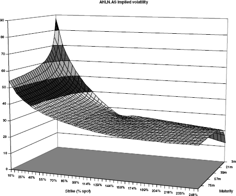
FIGURE 6.1 Ahold implied volatility as of December 2005, across a wide range of strikes and up to 7y maturity.

We therefore have a PDE in one spatial variable to solve for the single-name EDS. For a time-dependent protection payment R(t), the PDE we solve in a local volatility model with deterministic default risk is

The significant term in this is, of course, the inhomogeneous source term introduced by the presence of jumps.

A Worked Example: Ahold As an example, we select for study a five-year EDS written on Ahold (Reuters code AHLN.AS) with a barrier at 50% (of the share's traded price at the inception of the trade). (Ahold is a group of food retail and food service operators listed on Euronext and other exchanges.) As of December 2005, the credit default swap curve for this company was rising steeply from around 20bps for a one-year CDS to around 110bps at five years. With this information and market implied volatilities (shown in figure 6.1), we can calibrate a local volatility for the stock, given the possibility of jump to zero, using the procedures of chapter 8. The results of the calibration procedure are shown in figure 6.2.

The figure shows the relative error in European option prices after the calibration, that is, the difference between prices calculated in a local volatility model and market prices inferred from implied volatilities, divided by the price of the stock:

FIGURE 6.2 The local volatility calibration error on European option prices as a fraction of spot. The peak indicates the onset of arbitrage in the data.

The graph indicates that the majority of the region displayed calibrates to within ±10 basis points, regarded as reasonably acceptable. However, there is a pronounced peak at longer maturities and at spot prices below about 50% of the prevailing traded price. This is not an error in the calibration: It indicates the onset of arbitrage between the implied volatilities and the CDS curve used in the calibration. We can think of this in the following way:

For a constant volatility of the diffusion process, the presence of default risk makes puts more expensive as it raises the conditional (on no default) forward while at the same time introducing a likelihood of a maximum payout from the put. (The calibration options are taken to be riskless, perhaps exchange-traded, options on a risky share.) It also raises the call price: the increased forward contributing positively to the price while the probability of default before maturity resulting in a zero payout acts in the opposite way. Call-put parity is still required to hold, as the effect of default risk on the distribution at maturity is simply to change its form by introducing a peak at S_T = 0. (Throughout, we are considering that default results in the share price dropping to zero.) The local volatility calibration tries to compensate for this price-increasing effect of the credit by lowering the diffusion volatility to preserve the observed market price. If a near-zero local volatility cannot reproduce the calibration prices, then the data are arbitrageable.

We may value the EDS in a finite difference lattice scheme and use this to look at the price as a function of spot at the t = 0 time step of the grid.³ In the interests of simplicity, we will, in the following, drop the time variation of the protection payment caused by the accrued coupon. No essential features of the protection leg are lost.

FIGURE 6.3 A 5y EDS on AHLN.AS vs. share price. The asymptote is the value of a default protection written on the stock.

Figure 6.3 plots only the protection leg of the EDS. Note that, since the plot is taken from a single FD grid, the local volatility model is assumed valid, inasmuch as the local volatility surface is held constant rather than the implied surface. (See section 1.2.1 and remark 1.2.1 for reasons why keeping the implied surface constant between plots, and recalibrating local volatility each time, is inappropriate.) The graph shows an asymptote, which is the value of a pure default protection calculated according to

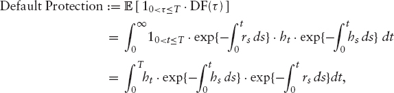
this being the value of a payment of one at the time of default, if default occurs before a maturity T.⁴ Although not visible in the graph, there is a small offset between the analytic default protection value and the limiting EDS leg value. This decreases slowly with increasing the number of time steps in the FD grid.

Were we to model the protection leg of the EDS on a default-free underlying, we would call it a deep out-of-the-money American Digital put,⁵ and the asymptotic

FIGURE 6.4 The vega and CDS curve sensitivity of the protection leg across a reasonably wide range of spot prices, showing regions of predominant equity sensitivity and credit sensitivity. The asymptote is the CS01 of the pure default protection.

value as S → ∞ would be zero, in contrast to figure 6.3. The only way in which such a structure can yield value to the holder, in the default-free model, is by the stock diffusing across the barrier. Contrast this with the EDS default protection leg on a risky underlying where the protection buyer can receive a payout either if diffusion carries the stock to the barrier or if default carries the stock clean through the barrier. Both possibilities contribute value to the structure, in amounts according to the distance of the asset from the barrier relative to the general level of its volatility and to its hazard rates. Accordingly, we can identify the two regimes in which the EDS can exist, and call them diffusion dominated and default dominated, corresponding to the cases where most of the value comes from the possibility of the stock diffusing to the barrier, and to the converse case where it mostly comes from the possibility of default.

We can quantify these notions by looking at the equity and credit sensitivities of the protection leg. We do so for our example Ahold EDS.

Figure 6.4 shows the vega and CDS curve sensitivity of the protection leg, in isolation, over a wide range of share prices around the prevailing traded price. The vega looks qualitatively very similar to the American Digital: necessarily zero at the barrier, positive elsewhere, and tending to zero as S → ∞ and the probability of diffusion to the barrier consequently vanishes. The sensitivity to CDS rates (known as CS01) tends to a nonzero asymptote as S → ∞: this is the CS01 of the pure default protection, as expected. The regions in which one sensitivity is substantial and the other negligible serve to identify the diffusion dominated and default dominated regions.

The negative CS01 near the barrier is at first sight counterintuitive: We plot it on an expended horizontal scale and a greatly expanded vertical scale in figure 6.5. The expectation is that increased CDS rates implies increased probability of default before maturity, increased value and positive CS01. This is indeed the case far from the barrier.

FIGURE 6.5 The CDS curve sensitivity of the EDS protection leg in the diffusion-dominated region near the barrier.

We can, however, understand how this intuition fails by noting that increased hazard rates increase the drift of the asset (the convection term in (6.30)) and so tend to bring it further from the barrier early in the lifetime of the structure. It is precisely in the diffusion-dominated region near the barrier that this is critical, where the likelihood is that the asset will diffuse to the barrier before it defaults. Increased drift lessens this likelihood, or lengthens the expected time before the barrier is breached. The negative CS01 indicates that this is more significant than the increase in the probability of breaching the barrier due to a default given that in this region any default is likely to occur after the barrier is hit.

6.8 CONCLUSION

In this chapter we have presented a modeling framework suitable for equity- and credit-sensitive structures. The main problem we face when it comes to pricing these structures is liquidity. Indeed, the scarcity of the data especially from the credit point of view makes it difficult to calibrate any model no matter how good that model.

While convertible bonds (see chapter 4, in the context of equity-interest rate hybrids) remain the most liquid and popular hybrid structure, we have witnessed lately a surge in new hybrid structures, such as the equity default swap.