CHAPTER 7

Copulas Applied to Derivatives Pricing

7.1 INTRODUCTION

In this chapter, we highlight the importance that copulas have gained in derivatives pricing in the last decade. This is due mainly to the growth seen in the credit derivatives markets. Indeed, basket default swaps, CDO tranches, and all correlation structures are often priced and risk managed using the copula technology. Copulas have been used widely in the insurance business, and the transition to the credit derivatives world was natural, as the latter is often thought of as an insurance business on the default of companies.

This chapter is organized as follows: First, we tackle copulas from a theoretical point of view by presenting various properties and families of copulas. We present as well the copula of a stochastic process highlighting the time dependency, or autocorrelation, induced by a process. Second, we look at some applications to derivatives pricing. We start by presenting the factor copula technique, which enables us to reduce dimensionality of the problem and find semiclosed-form solutions for various derivatives contracts. Last, we apply the previous approach to the pricing not only of credit derivatives but some popular multiunderlying equity derivatives, precisely collateralized debt obligations, basket default swaps, and Altiplanos.

7.2 THEORETICAL BACKGROUND OF COPULAS

7.2.1 Definitions

Definition and Sklar Theorem

DEFINITION 7.2.1 A copula is an n-dimensional function C: [0, 1]ⁿ → [0, 1], which has the following properties:

• C is increasing in each of its coordinates u_k for k ∈ {1, 2, …, n }.
• C(u) = 0 if at least one of the coordinates of the vector u is equal to 0.
• C(u) = u_k if all the coordinates of u but u_k are equal to 1.
• for every x, y ∈ [0, 1]ⁿ, such that x ≤ y¹. The volume of the hypercube H = [x₁, y₁] × [x₂, y₂] × … × [x_n, y_n], V_C(H) is non-negative, where

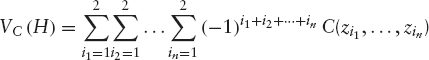
where z_ij = x_j if i_j = 1 and z_ij = y_j if i_j = 2 for j ∈ {1, …, n}.

From the above definition, we can conclude that a copula is a multidimensional distribution with uniform marginals. The following theorem proves to be at the heart of the copula theory and its applications.

THEOREM 7.2.1 (Sklar) Let F be an n-dimensional distribution function with marginals F₁, F₂, …, F_n, then there exist an n-dimensional copula C, such that

And if F₁, F₂, …, F_n are continuous, then C is unique.

REMARK 7.2.1 Let C be the copula of the random variables X and Y. Any increasing transformation of (X, Y) has the same copula C.

Frechet Bounds

THEOREM 7.2.2 Let C be a two-dimensional copula; we have the following result:

This result is straightforward: Due to monotonicity we have C(u, v) ≤ C(u,1) = u and C(u, v) ≤ C(1, v) = v. On the other hand, let H = [u, 1] × [v, 1]; we have V_C(H) ≥ 0, which implies C(u, v) ≥ u + v − 1, the positivity of C completes the proof.

W(u, v) = max(u + v − 1, 0) and M(u, v) = min (u, v) are called Frechet bounds. The Frechet bounds also exist in the multidimensional case and are given as follows:

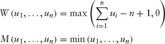
(u₁, …, u_n) ∈ [0, 1]ⁿ, n ≥ 2.

Another well-known and useful copula is the independence copula defined as follows:

REMARK 7.2.2 W is not a copula for n ≥ 3. Indeed, consider This means that condition 4 in the definition above is violated.

Conditional Distributions and Partial Derivatives The partial derivatives of a copula function are closely linked to the concept of conditional expectations. This proves to be very useful when sampling random variables whose dependency is described by a copula function. The heuristic argument comes from the following computation: Consider the probability measure Q and two random variables x₁ and x₂ with distribution functions F₁ and F₂ respectively and a joint distribution F.

The multidimensional density² f is linked to the copula function as follows:

where c(u₁, u₂, …, u_n) is the copula density.

7.2.2 Measures of Dependence

Concordance

DEFINITION 7.2.2 The realizations (x₁, y₁), and (x₂, y₂) of two random variables X, Y are said to be concordant if (x₁ − x₂) × (y₁ − y₂) ≥ 0, and discordant if (x₁ − x₂) × (y₁ − y₂) ≤ 0.

Kendall's Tau

DEFINITION 7.2.3 In a discrete space, if we call (x₁, y₁), (x₂, y₂)….(x_n, y_n) the possible realizations of two random variables X, Y. Let note c be the number of concordant pairs and d the number of discordant pairs. The Kendall's τ for this sample is defined as follows:

In the general case, Kendall's τ is defined as the probability of concordance minus the probability of discordance. Indeed, let (X₁, Y₁) and (X₂, Y₂) be two independent vectors with the same joint distribution function as (X, Y); we have

THEOREM 7.2.3 Let (X₁, Y₁) and (X₂, Y₂) be independent vectors with continuous random variables with joint distributions F₁ and F₂, respectively, with common marginals for F_X and F_Y. Denote C₁ and C₂ the corresponding copulas such that F₁(x, y) = C₁(F_X(x), F_Y(y)) and F₂(x, y) = C₂(F_X(x), F_Y(y)). If we define as the difference between the probabilities of concordance and discordance of(X₁, Y₁) and then

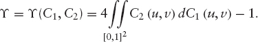
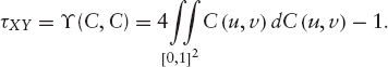
In the case of two continuous random variables X, Y whose copula is C, the Kendall's τ is given by

Spearman's Rho The Spearman's rho dependence measure is also based on concordance and discordance concepts.

DEFINITION 7.2.4 If we take now three independent random vectors (X₁, Y₁), (X₂, Y₂), and (X₃, Y₃) with the same joint distribution F, the Spearman's rho is defined as the difference between the probability of concordance and the probability of discordance of the two random vectors (X₁, Y₁) and (X₂, Y₃):

THEOREM 7.2.4 For continuous random variables X and Y whose copula is C, the Spearman's rho is given by

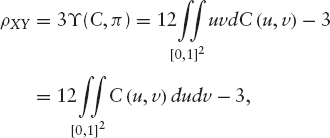
where η is the independence copula introduced previously.

Tail Dependence It is well known that the Gaussian copula, the most used one in the financial industry, fails to capture tail dependencies as its tails flatten very quickly. On the other hand, when dealing with fat-tailed distributions we want to know how well we capture the dependency between those extreme values. The two concepts of low tail dependency and up tail dependency have been introduced in order to measure the extreme values dependency as the number of financial contingent claims that depend on these values has risen dramatically in the last years. This has been triggered by the markets being marked with few extreme events, from the technology bubble to the corporate scandals and of course the terrorist attacks.

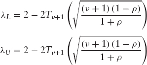
DEFINITION 7.2.5 Let X and Y be two random variables with cumulative distribution functions F_X and F_Y. The coefficients of upper and lower dependency are defined as follows:

provided, of course, that these limits exist.

If λ_L ∈]0, 1] (λ_U ∈]0, 1]) then X and Y are said to be asymptotically dependent in the lower tail (upper tail), and if λ_L = 0 (λ_U = 0), they are said to be asymptotically independent in the lower tail (upper tail).

We can show using the Base rule and the relationship between the survival function³ S(x, y) of (X, Y) and the cumulative distribution functions of X, Y and (X, Y) that

7.2.3 Copulas and Stochastic Processes

Some properties of stochastic processes can be characterized by their finite-dimensional distributions and therefore by copulas. Unfortunately, many of the stochastic process concepts are stronger than the finite dimensional distributions. In this paragraph, we focus on some well-known Markov⁴ processes. We define the copula of a Markov process X as being the copula C^{s, t} of X_t and X_s.

The Copula of a Brownian Motion From the definition of a Brownian motion we know that for t > s and x, y real numbers, we have

where N is the cumulative distribution function of a standard normal distribution variable.

Exploiting the relationship between the conditional expectation and partial derivatives of a copula we can write

where F_s and F_t are the cumulative distribution functions of W_s and W_t, respectively, and f_s is the density of W_s. Hence

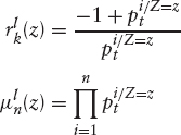
We therefore can express the copula as follows:

We have used The copula density is then given by

where φ is the density of a standard normal variable.

REMARK 7.2.3 A geometric Brownian motion is an increasing transformation of its underlying arithmetic Brownian motion; therefore, they have the same copula.

Copula of a Continuous Martingale By employing a time change we can link the copula of a martingale to that of a Brownian motion. This is possible only for martingales whose bracket goes to infinity when time goes to infinity.

THEOREM 7.2.5 Let X_t be a (Q, F_t) local martingale with deterministic bracket such that X₀ = 0 and a.s. Define T_t and B_t as follows:

B_t is an F_Tt Brownian motion and X_t = B_<X>t, and its copula is given by

The Copula of an Ornstein-Uhlenbeck Process: The OU process is defined on (Q, F_t) as follows:

where W_t is standard F_t Brownian motion and λ, σ > 0. Solving the above SDE we get

We can apply the above theorem to m_t = r_te^λt − r₀. We have and the copula of the process m_t is given by

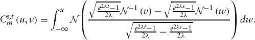
m_t is a monotone transformation of r_t and therefore has the same copula. We can note that the OU copula depends on λ but not on σ. On the other hand, when λ goes to zero, the OU copula is reduced to the Brownian motion copula. This is not surprising, as the process itself reduces to a Brownian motion. Whereas when λ goes to infinity, the OU copula tends to the independence copula π.

7.2.4 Some Popular Copulas

In this section, we present some copulas widely used in practice. They are appealing for their analytical and numerical tractability. Indeed, the Gaussian copula is used almost everywhere in the financial literature even if its use is most of the time implicit as we mention geometric Brownian motions and multidimensional log-normal distributions without using the word copula. It belongs to the family of elliptic copulas. Another family of widely used copulas is the Archimedean copulas.

Elliptic Copulas

Gaussian Copula

DEFINITION 7.2.6 The Gaussian copula is defined as follows:

where Σ is a correlation matrix, N_n,Σ is the standard n-dimensional normal distribution with correlation matrix Σ, and N⁻¹ is the inverse cumulative distribution function of a standard one-dimensional normal variable.

The corresponding copula density is given by

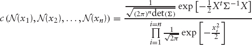
with X^t = (x₁, x₂, …, x_n). This leads to (N(x_i) = u_i)

where U^t = (N⁻¹(u₁),N⁻¹(u₂), …,N⁻¹(u_n)) and I_n is the identity matrix. The tail dependency parameters in the two-dimensional case are given as follows:

This concludes that the bivariate Gaussian copula does not exhibit tail dependency.

Student Copula (t-Copula)

DEFINITION 7.2.7 The t-copula is characterized by a correlation matrix Σ and a parameter ν called degree of freedom. It is defined as follows:

where T_{ν, n,Σ} is the n-dimensional student distribution with correlation matrix Σ and number of degrees of freedom ν, and is the inverse cumulative distribution of a student random variable with ν degrees of freedom. The corresponding copula density is given by

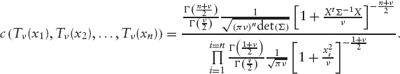
Changing variables and denoting T_ν(x_i) = u_i and leads to

where the Γ function is defined as follows:

The tail dependency parameters for the bivariate t-copula with linear correlation ρ can be shown to be:

It can be seen that a bivariate t-distribution exhibits tail dependency, in contrast with the bivariate Gaussian copula.

Archimedean Copulas

DEFINITION 7.2.8 Let φ be a strictly decreasing continuous function from [0, 1] to [0, +∞] such that φ(1) = 0. φ^[−1], the pseudo inverse of φ, is defined as follows:

if φ(0) = +∞, we have φ^[−1] = φ⁻¹.

THEOREM 7.2.6 Define the function C from [0, 1]² to [0, 1] such that C (u, v) = φ^[−1] (φ(u) + φ(v)). C is a copula if, and only if, φ is convex.

For a proof of this theorem, please refer to Nelson [133].

A generalization of this result defines the Archimedean⁵ copula in the multidimensional case.

The function φ is called the generator of the copula, and if φ(0) = +∞, φ is called a strict generator and the corresponding copula a strict Archimedean copula.

Examples:

• The independence copula Π is a strict Archimedean copula: indeed, π (u, v) = uv = exp (−[− ln u − ln v]), so define φ (x) = − ln (x) for x ∈ [0, 1]. We therefore have φ(0) = +∞ and π(u, v) = φ⁻¹ (φ(u) + φ(v)).
• Similarly, we can show that the Frechet boundary W, in the two-dimensional case, is also an Archimedean copula with φ(x) = 1 − x for x ∈ [0, 1].
• Considering with α ∈ [−1, +∞[{0} we have C(u, v) = φ^[−1] which is called the Clayton copula, and it is a strict copula if α > 0.

MinMax Copula In this section, we derive the copula of the minimum and maximum of n iid random variables X₁, X₂…,X_n with a distribution function F. We know that the distribution function of the order r (meaning that we order the variables from 1 to n and select the one of order r, which is similar to what we do with default times when trying to price an r-to-default basket) is given by

The minimum m_X and maximum M_X therefore have the following distributions:

On the other hand, we have the joint distribution of m_X and M_X given as follows:

By solving the equation C_mM (F_mX (x), F_MX (y)) = F_m,M (x, y) we get to the following expression for the MinMax copula of n iid random variables:

This copula is linked to the Clayton copula mentioned above. Indeed, if we consider the Clayton copula C_α with we can write

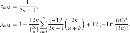
We can also note that when n goes to +∞, the MinMax copula approaches the independence copula π. Moreover, the Kendall's τ and Spearman's ρ for the MinMax copula are given by

7.3 FACTOR COPULA FRAMEWORK

The copula is only a way to separate the dependency structure (the copula) from the distribution of each random variable (the marginals). When it comes to pricing multiasset derivatives in practice, the dimension of the distribution of the copulated assets is generally high, and Monte Carlo simulation is the only applicable numerical method. There is nothing wrong with using Monte Carlo to price multiasset structures; however, as these structures become commoditized and traded in large volumes, the need for quicker methods becomes a necessity in order to deal with the volume. Another interest in faster pricers is the fact that they enable us to extract much more useful information from these structures such as greeks.

In order to tackle the dimensionality problem, factor copulas have been introduced. The idea is to factor the correlation matrix such that it depends only on few factors that explain a large percentage of the whole variance. This is similar to performing a Principal Component Analysis (PCA) on the correlation matrix.

The approach presented below is the one-factor Gaussian copula framework, a setting that is particularly well suited for high dimensional problems. The idea is that we choose a common factor that explains the dependency between n random variables such that they are independent conditionally on the common factor.

Let's define a series of hitting times τ^k with k ∈ {1, …, n}, and n being the number of assets. The hitting time could be the time to default of a credit name or the first time a stock hits certain level:

where L^k is the barrier related to the asset S^k that prevails at time t. The joint distribution function of the hitting times is

which can be modeled using the Gaussian copula thus:

where N_n,Σ is the n-dimensional Gaussian distribution with correlation matrix Σ, and F_i(t_i) = Q(τⁱ < t_i) is the distribution function of τⁱ for i ∈ {1, …, n}. Note that we have here chosen the copula function for the hitting times to be a Gaussian copula. It is a modeling choice and not something that could be derived. By construction, the vector (N⁻¹(F₁(τ¹)), …,N⁻¹(F_n(τⁿ))) is a Gaussian vector with a correlation matrix Σ.

Let (X₁, …, X_n) be a Gaussian vector, where X_k ≡ N⁻¹(F_k(τ^k)), k = 1,…,n. In the following, we consider a special case of a one factor copula representation, where

and Z, k = 1, …,n are independent standard Gaussian random variables. On the other hand, ρ_k ∈ [−1, 1], k = 1, …, n are calibrated to the initial correlation matrix Σ.

Denoting by and exploiting the independence assumption, matrix we readily get

The joint distribution and copula functions are then given by

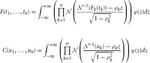
where is the Gaussian density.

In the following section we are going to take advantage of source of the foregoing results in order to price semianalytically some complex structures that otherwise require lengthy Monte Carlo simulations to price and risk manage. We have chosen a well-known equity derivative structure named Altiplano, a very popular credit derivatives structures called collateralized debt obligations (CDOs), and basket default swaps.

7.4 APPLICATIONS TO DERIVATIVES PRICING

7.4.1 Equity Derivatives: The Altiplano

A family of equity derivatives structures called mountain range options arose during the 1990s and subsequent years. They are a series of path-dependent options on a basket of underlying assets. Exotic mountain names have been assigned to these structures like Altiplano, Himalaya, Atlas, Everest, Annapurna, Etna, and many more.

These structures are usually written on many underlying assets, and Monte Carlo simulation is the only suitable numerical method to price them. Unfortunately, this method shows its limits when it comes to live risk management. Indeed, because of the large dimension of the portfolio, the number of computed quantities, that is, price, and different greeks grows rapidly, it becomes intractable to have quick and accurate results.

In the remainder of this section, we focus on the pricing of the Altiplano structures using the factor copula framework presented before. We therefore start with a quick reminder of an Altiplano payoff, then prepare the ingredients for the factor copula approach by computing the cumulative distribution functions for a currently running period and a period starting in the future. A semianalytical solution is derived for the price of this structure.

The structure we are interested in is a multiasset, multibarrier option that pays a series of coupons depending on the number of assets crossing the barriers and on the barrier period. No underlying is removed throughout the life of the product.⁶

We are given

• n starting assets prices

  

• The corresponding correlation matrix Σ of these assets
• A set of m monitoring periods [T₀, T₁] …[T_m−1,T_m]
• A barrier matrix being the barriers applying to each
  asset serving each monitoring period
• A maturity date T
• Amatrix of coupon payments, the structure pays at

  T_i the coupon where j is the number of assets which breached their respective barriers during the period [T_i−1, T_i].

  Normally, one has and

  The coupon payments are made at the end of each barrier period.

  We define the n stopping times for each period l, hence is the first time when asset Sⁱ hits the barrier for the period l. Let N^l be the number of assets that hit the given barriers, that is,

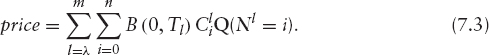
Therefore, the value at time 0 of an m period, n-underlying Altiplano that pays at maturity is

In order to use the factor copula approach, we will need to compute the marginal distribution functions of the hitting time, and this is the subject of the next section.

Cumulative Distribution Functions of the Hitting Times

Current period The current period is a barrier period that contains the valuation sale. We are working in the n-dimensional correlated Black-Scholes model, that is,

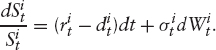
The hitting time, of a certain barrier LS₀, for an underlying S_t is defined as follows:

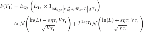
We have to compute the following quantity F(T₁) = Q(τ < T₁):

α_s is defined as follows:

where r_s is the short rate and d_s is the dividend and repo rates and σ_s is the volatility function of S_t.

L_t is defined as follows:

and

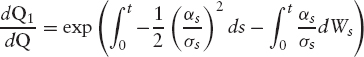
Girsanov theorem tells us that is a Brownian motion under Q₁. Define the following quantities:

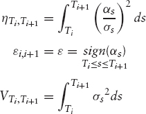
Assuming that α_s has the same sign either positive or negative throughout the period (the same assumption is made for forward periods), we have the following result:

Forward period For a forward period [T_i, T_{i +1}], the computation is similar.

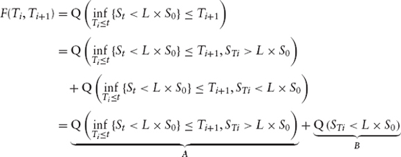
The second term B is easy to compute:

Following the same steps of the computation in the previous paragraph we have:

where N₂ is the bivariate normal distribution function and x₁, y₁, x₂, y₂, ρ and fact are given by

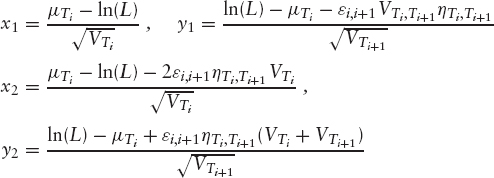
where

Up to this point we have prepared the main ingredients for the copula approach. In the next paragraph, we apply this in order to derive a semiclosed solution for the structure presented above.

Pricing of Altiplanos In order to compute the price in (7.3), all we need to do is to compute the probabilities Q(N^l(t) = k) (k hits for the period l).

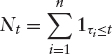
Recall that the counting process associated with the number of hits up to time t for the period l.

The probability generating function of N^l(t) is given by

Recall

Using the iterated expectations theorem, Ψ_N^l(t) can be rewritten as

where the last equality stems from a formal expansion of

Note that we have dropped the index l from the probabilities to ease the notation.

Using the vieta's formulas, which link the roots of a polynomial to its coefficients, we can express μ_k(z) as a function of

where

The probability of k hits by time t is thus given by

and the price in (7.3) is given as follows:

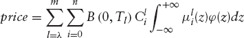
This integral maybe evaluated using a simple quadrature and it reduces the computation time massively.

In the following section, we focus on the application of the above approach to multiname credit derivatives, specifically CDOs and basket default swaps.

7.4.2 Credit Derivatives: Basket and Tranche Pricing

The extensive application of copulas in the financial industry is in large part due to the development of the credit derivatives market. In this section, we present an approach to pricing the well-known CDOs and basket default swaps in the factor copula framework presented above in the same way we did for Altiplano.

Pricing of CDO Tranches

Introduction Collateralized Debt Obligations belong to a class of securitized products called Asset Backed Securities (ABS). These are securities backed by pools of assets which range from corporate bonds, bank loans, catastrophe bonds, emerging market securities, credit cards, or various types of mortgage securities. These securities are the property of a special purpose vehicle (SPV) which issues a variety of equity and debt notes (tranches). Typically, the SPV issues an equity, junior, mezzanine, and senior tranches plus sometimes a super-senior tranche. The fundamental difference of these tranches lies in the risk they bear as the repayment of both interests and principal is done in a given order and the first losses are borne by the equity tranche.

The SPV is called a CDO which also refers to the various notes issued by the SPV, this leads to the known circular phrase “a CDO issues CDOs.” These are bought by investors looking to gain an exposure to a diversified portfolio of underlying assets without having to buy each asset individually, and to obtain a higher return than is available on other securities of equivalent credit rating.

The motivations behind participating in the CDO market are different for both the originator and the investor. Banks for example, or any other holder of assets, aim at shrinking the balance sheet, therefore reducing the required regulatory capital, or economic capital. Investors, on the other hand, are looking for both investment and arbitrage opportunities. These motivations coupled with the source of the underlying assets allow for a classification of CDOs into Balance Sheet and Arbitrage CDOs.

Synthetic CDOs Synthetic CDOs are similar to ordinary CDOs, or cash CDOs, except that their portfolios are constituted of Credit Default Swaps (“CDS”) rather than actual bonds or loans. In a CDS, one counterparty pays a premium to a second counterparty in exchange for a contingent payment should a defined credit event occur such as the reference entity going into default. This way the CDO gains exposure synthetically to a reference credit entity without purchasing a bond or a loan. An analogy can be drawn with insurance where one party pays regular premiums against the protection, by the other party, against potential coverage losses.

The sophistication of synthetic CDOs has reached another level as the underlying portfolio is customized to include CDO notes (CDO², CDO squared), and this works in the same way as a standard CDO structure. Leveraged super senior and CPPI on CDO tranches constitute the latest innovations in the field of CDOs.

Synthetic CDOs offer access to a more diversified portfolio of assets and a larger number of assets than Cash CDOs. They also create a cheaper capital structure, leading to higher equity returns and higher portfolio quality.

Default Leg of a CDO Given a pool of n credit names with recovery rates R_i and nominals N_i, i ∈ {0, …, n}. We denote by τ_i the default time of credit name i. We assume the recovery rates are known beforehand. Define L_t the cumulative loss of the portfolio at the time t:

where is the loss if the name i defaults before time t, and Lⁱ = (1 − R_i)N_i. We assume that interest rates are deterministic.

We consider a CDO tranche where the default leg pays losses borne by the above portfolio and which are in excess of K₁ and not more than K₂ (K₁ < K₂). The payoff of the tranche is therefore given as follows:

K₁ = 0 corresponds to the equity tranche, corresponds to the senior tranche and finally K₁ > 0 and corresponds to the mezzanine tranche.

For a maturity T, the price of the default leg is the expectation of the sum of all default payments before T. It is given as follows⁷:

Using integration by parts we have:

where f( 0, t) is the instantaneous forward rate defined as follows: f (0, t) =

For simplification we consider the case where all the names have the same nominal and recovery rate; this is called a homogeneous portfolio (Lⁱ = L, for all i’s). Denote by k₁ and k₂ the number of defaults that correspond to the losses K₁ and K₂, respectively.

Within the one-factor Gaussian copula framework presented above, we have

where μ_k is the coefficient of u^k in the moment-generating function.

Fixed Leg The fixed leg is a risky coupon-bearing bond with a notional equal to the notional of the tranche K₁, K₂. Hence, we have the following expression:

where t_is, i ∈ {1, … p}, are the payment dates and s is the fixed premium paid at each payment date.

The CDO spread is the value of s that makes the default leg equal to the fixed led and is given by

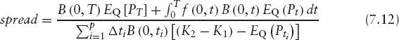
Note that in the above computation we have omitted for simplicity the accrual payment that could be added to the fixed leg in the event that the default happens between two premium dates.

This comes down again to the computation of the probabilities Q(N_t = m), which is, as explained before, very easy to compute within the factor copula framework.

We can therefore compute the prices of different tranches in a CDO by numerical integration. The generalization to a nonhomogenous portfolio is straightforward.

Pricing of Basket Default Swaps Another structure that provides similar credit protection to CDO tranches is a Basket Default Swap. A basket swap is similar to single name credit default swap except that it offers protection against a number of credit entities (2 to 25 or 30 names) rather than a single entity. These can be structured in a way that offers investors access to different risk profiles depending on their risk appetite, and protects against different ranges of portfolio losses.

In a First to Default (FTD) swap, the protection buyer is only protected against the losses incurred on the first default and the contract is terminated after this event. In a Second to Default swap, the protection buyer is protected against the losses incurred on the first and second defaults but not the third with the contract being terminated after the second default. In a Ninth to Default swap, the protection buyer is protected against the losses incurred on the first nine defaults but not the tenth. These structures would be similar to the equity tranche, mezzanine tranche, and senior tranche of a CDO, respectively.

The success of these structures stems from the fact that they offer the investor higher spreads than the underlying single name credit default swaps. However, this spread depends on the level of correlation between the reference credits constituting the basket.

Pricing a k^th to Default Basket As in the case of CDOs, we consider a pool of n credit names with recovery rates R_i and nominals N_i, i ∈ {0, …, n}. We denote by τ_i the default time of credit name i. We assume the recovery rates are known beforehand. Let N_t be the counting process:

We also assume for simplicity that we have a homogeneous portfolio (R_i = R, and N_i = N), and we have therefore Lⁱ = (1 − R) N = L where Lⁱ is the loss incurred if the name i defaults. We also assume that interest rates are deterministic.

As mentioned before, the k^th to default basket is swap that provides a protection against defaults up to the k^th. We therefore are interested in the distribution of τ^(k), which is the k^th default time.

We can write:

The Default Leg The default leg denoted DL is computed as follows:

where f^τ(k) (t) is the density function of τ^(k) given by

Within the one factor Gaussian copula framework, F^τ(k) (t) is given as a sum of Q(N_t = m), k ≤ m ≤ n, where, as explained before:

where μ_k is the coefficient next to u^k in the moment-generating function.

Note that (7.13) could be written as follows:

Integrating by parts we get:

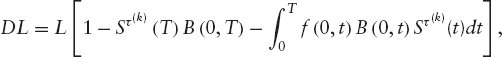
where s^τ(k) (t) is the survival probability density given by

and S^τ(k) (t) by

Therefore, depending on the number of terms in the sum, we can use one or the other (survival or default) to ease computations.

The Fixed Leg As with the CDO, the fixed leg of a basket default swap is basically a risky coupon bond. Hence, we have the following expression:

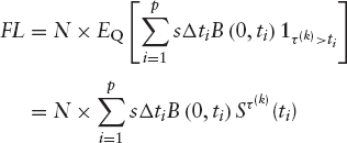
where t_is, i ∈ {1,…,p}, are the payment dates, Δt_i = t_i − t_i−1, and s is the fixed premium paid at each payment date.

As with the CDO, the k^th to default basket default swap spread is the value of s that makes the default leg equal to the fixed led and is given by

Again, we have omitted for simplicity the accrual payment that could be added to the fixed leg in case the default happens between two premium dates.

This comes down again to the computation of the probabilities Q(N_t = m), which is, as explained before, very easy to compute within the factor copula framework.

7.5 CONCLUSION

Copulas have found many applications within the field of financial derivatives. Their application is not limited to equity or credit derivatives. Copulas are also used for risk management purposes as the calculation of risk limits for large portfolios poses problems similar to the pricing of CDOs and Altiplanos. They we also applied in interest rates derivatives for structures like CMS spread options, and the field of hybrid derivatives.