1.1 Getting Started

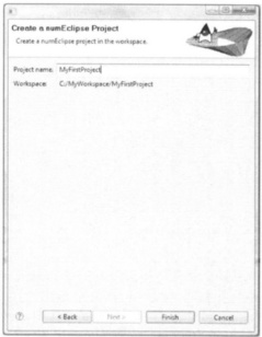
In this section, we will introduce the numEclipse working environment. We will learn how to create a numEclipse project. We will review the user interface including numEclipse perspective and views. Installation of numEclipse plug-in requires the latest java runtime environment and Graphical Modeling Framework (GMF) based eclipse installation. A step by step guide for installation and configuration is provided on the project website (http://www.numeclipse.org). Once the plug-in is successfully installed, configured and verified, we are ready to create our first project. This two step process is described as follows. Select eclipse menu File → New → Project. It will bring up New Project dialog box. Select the wizard numEclipse Project under the category numEclipse and click on Next button, as shown in figure 1.1. It will bring up the Project Wizard for numEclipse. Type the project name in the textbox and click on Finish button, as shown in figure 1.2. On successful completion of the above steps, you will see that a project has been created in your workspace. Also, you will notice that the Perspective is changed from Java to numEclipse, as shown in figure 1.3.

Before looking at the numEclipse perspective (figure 1.3), it is important to understand the project structure just created. The navigator view on the left of the perspective shows the project. It consists of two folders (i.e. “Interpreter” and “Source”) and a default interpreter default.i created under folder Interpreter. If the navigator view’s filter does not block resources files then you will also be able to see the project file created for the numEclipse project. The central area of the window shows the default, i interpreter. This is where most of the user interaction happens. Here you will type the commands and look at the results, as shown in the following listing (listing 1.1).

The area at the bottom of the perspective shows history view. This view keeps track of all the activities happening in the interpreter. This view has two parts; the area on the left of the history view shows the sequence number, date/time and the command in chronological order. The area on the right of the view shows the details of the command selected on the left, as shown in figure 1.4.

The cross × button on the top right of the view is used to clear the history view. It will erase all the entries in the view. A user can select the contents of the window on the right and copy it to the interpreter to run the command. The area on the right of the perspective is the memory view. This view shows all the variables in the memory of the interpreter. This view also has two parts. The part on the top shows the list of variables and their corresponding types. When a variable is selected in this part of the view, the corresponding value of that variable is shown in the bottom part of the view. Like the history view, the cross × button on the top right of the memory view is used to clear the memory. It will erase all the entries in the view.

It might seem like a lot of work for somebody who is new to scientific computing or more familiar with MATLAB. But, it must be remembered that this tool offers more than an interpreter and it is more geared towards scientific application development. There are a lot of benefits of project oriented approach even for an end user. Unlike MATLAB, you can open more than one interpreter at a time. Say you wanted to work on calculus, right click on Interpreter folder and create a simple file calculus, i. This will open another interpreter window in the center of the perspective. A project allows you to open as many interpreter windows you need. In MATLAB, you will have to launch a new instance of the application in order to get another interpreter window. The memory and history views are associated to the active interpreter. When you switch the interpreter window, the memory and history views will reflect the activity in the current active window. You can also save the session for each interpreter using menu File → Save. Next time when you launch the application, it will load all the variables and history from the saved session file.

1.2 Interpreter

numEclipse can be used in two modes; interactive and programming. In the interactive mode, we type the commands in the interpreter window and execute them as we go from one command to another. This mode is useful when you are experimenting with your algorithms or you are using the tool as a sophisticated scientific calculator. In the programming mode, you would write a set of commands / statements in a file and execute all the commands in the file together. The commands / statements in both modes are almost same, as they are based on the same language specification. In interactive mode, you have some additional commands specific for the interactive environment which is not applicable to the programming environment. The interpreter allows you to write and test mathematical expressions and small blocks of code. One can start typing the commands directly after the prompt > > as shown in listing 1.2.

It creates an array x with values from 0 to 10. Note that there is no need to declare or initialize a variable. The type of a variable is determined by the use and it could change with next command, as shown in listing 1.3.

Now, the type has changed to string and the same variable x has a value Hello World. Variable name should always start with a letter and it is case-sensitive. Each line that we type in the interpreter is captured by the history view and each new variable introduced in the interpreter is shown in the memory view. This could be used for the debugging purposes.

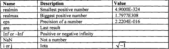
In the example shown in listing 1.4, an array t is created with values ranging from 0 to pi with the increment of 0.1. Here pi is a mathematical constant. You would notice that the output of the expression is not echoed back to the screen. This is due to the semicolon at the end of the line. numEclipse has some built-in variables and constants as given in table 1.1.

numEclipse has a very interesting feature which is not available in MATLAB/Octave. It allows you to define your own constants. Select eclipse menu Windows → Preferences, it will bring up the Preferences dialog box. On the left of the dialog box, expand the category numEclipse → Preferences and select Constants, as shown in figure 1.6. Here you can add or modify constants and they immediately become available in all the interpreter instances.

So it is important as part of configuration to define the constants required for your specific work.

Expression in listing 1.5 creates a new array y which contains the sin values of the previously defined array t. numEclipse provides integration with gnuplot. The steps to configure link to gnuplot are described on project website, plot command opens a gnuplot window if it is not already initialized and it draws a line plot of variable y versus corresponding values of t, as shown in following figure 1.7. Chapter 7 covers the plotting functions in detail.

1.3 Program

The interpreter allows running one statement at a time whereas a program contains a number of statements in a single file and runs all the statements at one time. A numEclipse program is a simple text file with m extension. It must reside under the Source folder. Programs could be organized by creating sub-folders within the Source folder to any level of hierarchy. In order to create a program, right click on the source folder and create a new simple file firstprog.m. Add the code in listing 1.6 to the file.

Once it is saved, it can be used from any instance of the interpreter. Either open up the default interpreter or create a new interpreter as described earlier. Enter the command in listing 1.7 to the command prompt.

The GNU Plot window is shown the following figure 1.8

You can use either the memory view on the right-hand side of the perspective to examine the value of variable h used in the program or you can just enter h on the prompt to get the value as shown in listing 1.8.

Note that the program does not have any structure like begin to indicate the start of the program or end to indicate the end of the program. It is just a collection of commands that you could also execute from the interpreter.