
Interpolation and Approximation
11.1 Interpolation
For practical use, it is convenient to have an analytical representation of the relationships between variables in a physical problem, and this representation can be approximately reproduced from data given by the problem. The purpose of such a representation might be to determine the values at intermediate points, to approximate an integral or derivative, or simply to represent the phenomena of interest in the form of a smooth or continuous function.
Interpolation refers to the problem of determining a function that exactly represents a collection of data. The most elementary type of interpolation consists of fitting a polynomial to a collection of data points. For numerical purposes, polynomials have the following advantages: they have derivatives and integrals that are themselves polynomials, and their computation is reduced to additions and multiplications only.
11.1.1 Polynomial interpolation
To begin with, consider the problem of determining a polynomial of degree one that passes through the distinct points (x0, y0) and (x1, y1). The linear polynomial
has the required property: it is easy to verify that P1(x0) = y0 and P1 (x1) = y1. To generalize the concept of linear interpolation to higher-degree polynomials, consider the construction of a polynomial of degree at most N that has the property
where points xn and yn are given. This polynomial is unique and may be represented in the form

Polynomial (11.2) is called the Nth Lagrange interpolating polynomial. For an evaluation of the interpolating polynomial at a single point x without explicitly computing the coefficients of the polynomial, the following Neville scheme is very practical. Firstly we define
then interpolating polynomials are determined according to the recursive relation
Representation (11.2) is very convenient for theoretical investigations because of its simple structure. However, for practical computations it is suitable only for small N. For large N the Lagrange factors ln(x) become very large and highly oscillatory. There is another representation of the interpolating polynomial that is more practical for computational purposes. We first need to introduce divided differences. Assume that N + 1 distinct points x0, …, xN and N + 1 values y0, …, yN are given. The zeroth divided differences are simply the values of yn:
The divided differences of order k at the point xn are recursively defined by

With this notation, the uniquely determined interpolating polynomial with property (11.1) is given by
Polynomial (11.4) is called the Newton interpolating polynomial. This polynomial can also be written in a nested form:
Thus, the value of the Newton interpolating polynomial at a point x can be calculated using the following algorithm (the Horner scheme):
As noted earlier, the Lagrange interpolating polynomial is a linear combination of Lagrange coefficients. Before implementing the function to calculate the polynomial, we implement the function to evaluate the Lagrange coefficient in the following. This function takes four arguments. The first argument is the value of x where we want to calculate the Lagrange coefficient. The second argument is a two column matrix with the first column containing the values of x and the second column containing y. The third argument, n, is the order of the coefficient and the last argument is the order of the polynomial.
In the following, we implement the function to evaluate Lagrange polynomial at a given value of x. The function takes similar parameter except we do not need the order of coefficients.
We apply the above function on the following set of data.

We apply the Lagrange polynomial method in the following to determine the curve representing this dataset.
11.1.2 Trigonometric interpolation
Periodic functions occur quite frequently in applications. These functions have the property f(x + T) = f(x) for some T > 0. For example, functions defined on closed planar or spatial curves may always be viewed as periodic functions. Polynomial interpolation is not appropriate for such functions, because algebraic polynomials are not periodic. Therefore, we turn to a consideration of interpolation by trigonometric polynomials. Without loss of generality we assume that the period T is equal to 2π. Assume that 2 N + l distinct points x0, …, x2N ∈ [0, 2π) and 2 N + 1 values y0, …, y2N are given. Then a uniquely determined trigonometric polynomial Qn(x) exists and it has the property
In the Lagrange representation, this polynomial is given by

When the interpolation points are equally spaced, representation (11.5) can be simplified. For an equidistant subdivision with an odd number 2 N + l of interpolation points
there exists a unique trigonometric polynomial
satisfying the interpolation property

For an equidistant subdivision with an even number 2 N of interpolation points
there exists a unique trigonometric polynomial
satisfying the interpolation property
Trigonometric interpolation polynomials (11.6) and (11.7) may be viewed as the discretized versions of the Fourier series, where the integrals giving the coefficients of the Fourier series are approximated by the rectangular rule at an equidistant partition.
An efficient numerical evaluation of trigonometric polynomials can be done analogously to the Horner scheme for algebraic polynomials. The recursion scheme has the form

starting with aN = aN and N = 0. It delivers
If we use bn instead of an and start with aN = bN and bN = 0, then recursion scheme (11.8) delivers
Hence the evaluation of a trigonometric polynomial at a point x can be reduced to the evaluation of sin(x) and cos(x), and 6 N additions and 8 N multiplications.
The trigonometric polynomial is a linear combination of Lagrange like trigonometric coefficients. Before implementing the function to calculate the polynomial, we implement the function to evaluate the trigonometric coefficients in the following. The implementation is very similar to the implementation in the previous section. This function takes four arguments. The first argument is the value of x where we want to calculate the coefficient. The second argument is a two column matrix with the first column containing the values of x and the second column containing y. The third argument, n, is the order of the coefficient and the last argument is the order of the polynomial.
In the following, we implement the function to evaluate the trigonometric polynomial at a given value of x. The function takes a similar parameter except that we do not need the order of coefficients.
We apply the above function on the following set of data.

We apply the trigonometric polynomial method in the following and determine the curve representing this dataset.
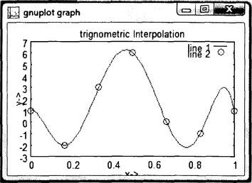
Figure 11.2
11.1.3 Interpolation by splines
When a number of data points N becomes relatively large, polynomials have serious disadvantages. They all have an oscillatory nature, and a fluctuation over a small portion of the interval can induce large fluctuations over the entire range.
An alternative approach is to construct a different interpolation polynomial on each subinterval. The most common piecewise polynomial interpolation uses cubic polynomials between pairs of points. It is called cubic spline interpolation. The term spline originates from the thin wooden or metal strips that were used by draftsmen to fit a smooth curve between specified points. Since the small displacement w of a thin elastic beam is governed by the fourth-order differential equation d4w/dx4 = 0, cubic splines indeed model the draftsmen splines.
A cubic spline interpolant s(x) is a combination of cubic polynomials (sn(x)(s(x) = ∪ sn(x)), which have the following form on each subinterval [xn, xn + 1]:
To determine the coefficients of sn(x), several conditions are imposed. These include
These conditions result in the system of linear equations for coefficients cn of cubic polynomial (11.9):

where Δxn = xn + 1 − xn The coefficient matrix of this system is a tridiagonal one, and it also has the property of diagonal dominance. Hence, the solution of this system can be obtained by the sweep method. Once the values of cn are known, other coefficients of cubic polynomial sn(x) are determined as follows:

11.2 Approximation of Functions and Data Representation
Approximation theory involves two types of problems. One arises when a function is given explicitly, but one wishes to find other types of functions which are more convenient to work with. The other problem concerns fitting functions to given data and finding the “best” function in a certain class that can be used to represent the data. We will begin this section with the latter problem.
11.2.1 Least-squares approximation
Consider the problem of estimating the values of a function at nontabulated points, given the experimental data in Table 11.1.
Table 11.1
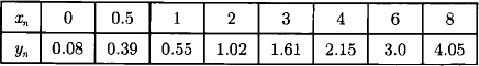
Interpolation requires a function that assumes the value of yn at xn for each n = 1, …, 11. Figure 11.1 shows a graph of the values in Table 11.1. From this graph, it appears that the actual relationship between x and y is linear. It is evident that no line precisely fits the data because of errors in the data collection procedure. In this case, it is unreasonable to require that the approximating function agrees exactly with the given data. A better approach for a problem of this type would be to find the “best” (in some sense) approximating line, even though it might not agree precisely with the data at any point.

Figure 11.1
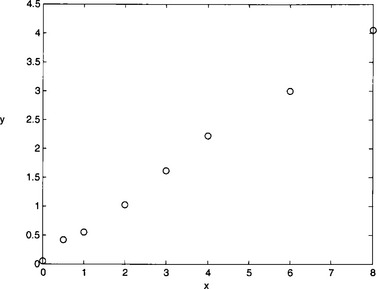
Figure 11.3 Graph of the values listed in Table 11.1.
Let fn = axn + b denote the nth value on the approximating line and yn the nth given y-value. The general problem of fitting the best line to a collection of data involves minimizing the total error
with respect to the parameters a and b. For a minimum to occur, we need
These equations are simplified to the normal equations
The solution to this system is as follows:
This approach is called the method of least-squares.
The problem of approximating a set of data (xn,yn), n = 1, …, N with an algebraic polynomial
of degree M < N-1 using least-squares is resolved in a similar manner. It requires choosing the coefficients a0, …, aM to minimize the total error:
Hence, the conditions ∂e/∂am = 0 for each m = 0, …, M result in a system of M + 1 linear equations for M + 1 unknowns am,

This system will have a unique solution, provided that the xn are distinct. We apply the above method on the following set of data.

There are 7 data points (N = 7) and we will use a 3rd order polynomial for least square approximation (M = 3). We build the following linear system of equations based on the least square method.

We solve the above system of equations in the following to find out the unknown values of a’s.
Once we know the polynomial coefficients, we could use the built-in polyval function to evaluate the polynomial for different values of the independent variable, x. We use this function in the following to generate the approximate polynomial values and create a plot showing the given data points and the approximating polynomial.
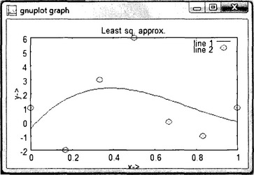
Figure 11.4
The approximating polynomial function nicely goes through the data points. The error could be reduced by increasing the polynomial order. But for the high order polynomial the curve shows oscillatory behavior so we could only use the low order polynomial.
11.2.2 Approximation by orthogonal functions
We now turn our attention to the problem of function approximation. The previous section was concerned with the least-squares approximation of discrete data. We now extend this idea to the polynomial approximation of a given continuous function f(x) defined on an interval [a,b]. The summations of previous section are replaced by their continuous counterparts, namely defined integrals, and a system of normal equation is obtained as before. For the least-squares polynomial approximation of degree M, the coefficients in
To determine these coefficients we need to solve the following system of linear equations

These equations always possess a unique solution. The (n,m) entry of the coefficient matrix of system (11.12) is

Matrices of this form are known as Hilbert matrices and they are very ill conditioned. Numerical results obtained using these matrices are sensitive to rounding errors and must be considered inaccurate. In addition, the calculations that were performed in obtaining the Nth degree polynomial do not reduce the amount of work required to obtain polynomials of higher degree.
These difficulties can, however, be avoided by using an alternative representation of an approximating function. We write
where φm(x) (m = 0, …, M) is a function or polynomial. We show that, by proper choice of φm(x) , the least-squares approximation can be determined without having to solve a system of linear equations. Now the values of am(x) (m = 0, …, M) are chosen to minimize

where ρ(x) is called a weight function. It is a nonnegative function, integrable on [a,b], and it is also not identically zero on any subintervals of [a,b]. Proceeding as before gives
This system will be particularly easy to solve if the functions m(x) are chosen to Satisfy
In this case, all but one of the integrals on the left-hand side of equation (11.14) are zero, and solution can be obtained as

Functions satisfying (11.15) are said to be orthogonal on the interval [a,b] with respect to the weight function ρ(x). Orthogonal function approximations have the advantage that an improvement of the approximation through addition of an extra term aM + 1φM + 1(x) does not affect the previously computed coefficients a0, …, aM. Substitution of
where x∈ [a, b] and ![]() in equations (11.13) to (11.15) yields a rescaled and/or shifted expansion interval.
in equations (11.13) to (11.15) yields a rescaled and/or shifted expansion interval.
Orthogonal functions (polynomials) play an important role in mathematical physics and mechanics, so approximation (11.13) may be very useful in various applications. For example, the Chebyshev polynomials can be applied to the problem of function approximation. The Chebyshev polynomials Tn(x) are orthogonal on [-1, 1] with respect to the weight function ρ(x) = (1-x2)− 1/2. For x∈ [–1, 1] they are defined as Tn (x) = cos(n arccos(x)) for each n≥ 0 or
The first few polynomials Tn(x) are
The orthogonality constant in (11.15) is an = π/2. The Chebyshev polynomial TN(x) of degree N≥ 1 has N simple zeros in [-1, 1] at
for each n = 1, …, N. The error of polynomial approximation (11.13) is essentially equal to the omitted term aM + 1TM + 1(x) for x in [-1,1]. Because TM + 1(x) oscillates with amplitude one in the expansion interval, the maximum excursion of the absolute error in this interval is approximately equal to |aM + 1|.
Trigonometric functions are used to approximate functions with periodic behavior, that is, functions with the property f(x + T) = f(x) for all x and T > 0. Without loss of generality, we assume that T = 2π and restrict the approximation to the interval [–π,π]. Let us consider the following set of functions

Functions from this set are orthogonal on [-π,π] with respect to the weight function ρ(x) = 1, and αk are equal to one. Given f(x) is a continuous function on the interval [-π,π], the least square approximation (11.16) is defined by
As cos(mx) and sin(mx) oscillate with an amplitude of one in the expansion interval, the maximum absolute error, that is max |f(x) − g(x)|, may be estimated by
The following function finds the coefficients for Chebyshev polynomial for a given input function argument and the degree of the polynomial.
The following function evaluates the Chebyshev polynomial for a given input vector containing polynomial coefficients and the value of x where the polynomial needs to be calculated.
We use the last two function implementations in the following program to determine the Chebyshev approximation of the exponential function ex for x ∈ [-1, 1].
This program generates the following plot which shows some of the points of the exponential function along with the curve obtained by the approximated Chebyshev polynomial. It is interesting to see how the curve neatly goes through the exponential function points.

Figure 10.7
11.2.3 Approximation by interpolating polynomials
The interpolating polynomials may also be applied to the approximation of continuous functions f(x) on some interval [a,b]. In this case N + 1 distinct points x0, …, xN∈ [a,b] are given, and yn = f(xn). First, let us assume that f(x) is defined on the interval [-1, 1], If we construct an interpolating polynomial, which approximates function f(x), then the error for this approximation can be represented in the form
where PN(x) denotes the Lagrange interpolating polynomial. There is no control over z(x), so minimization of the error is equivalent to minimization of the quantity (x-x)(x-x1)…(x-xN). The way to do this is through the special placement of the nodes x0,…, xN, since now we are free to choose these argument values. Before we turn to this question, some additional properties of Chebyshev polynomial should be considered.
The monic Chebyshev polynomial (a polynomial with leading coefficient equal to one) Tn⁎(x) is derived from the Chebyshev polynomial Tn(x) by dividing its leading coefficients by 2n−1, where n≥ l. Thus
As a result of the linear relationship between Tn⁎(x) and Tn(x), the zeros of Tn⁎(x) are defined by expression (11.17). The polynomials Tn⁎(x), where n≥ 1, have a unique property: they have the least deviation from zero among all polynomials of degree n. Since (x-x0)(x-x1)…(x-xN) is a monic polynomial of degree N + 1, the minimum of this quantity on the interval [-1, 1] is obtained when
Therefore, xn must be the (n + l)st zero of Tn + 1⁎(x), for each n = 0. …, N; that is, xn = xN + 1,n + 1⁎ This technique for choosing points to minimize the interpolation error can be extended to a general closed interval [a,6] by choosing the change of variable

to transform the numbers xn = xN + 1,n + 1⁎ in the interval [-1, 1] into corresponding numbers in the interval [a,b].
11.3 Exercises
It is suggested to solve one of the following three problems:
(a) Calculate coefficients of Lagrange interpolating polynomial that passes through the given points xn and yn (tables 11.2-11.7). Plot the polynomial together with initial data.
Table 11.2
| x | y |
| 0 | 0 |
| 0.2 | 0.3696 |
| 0.5 | 0.5348 |
| 1 | 0.6931 |
| 1.5 | 0.7996 |
| 2 | 0.8814 |
Table 11.3
| x | y |
| 0 | 0 |
| 0.2 | 0.1753 |
| 0.5 | 0.3244 |
| 1 | 0.3466 |
| 1.5 | 0.2819 |
| 2 | 0.2197 |
Table 11.4
| x | y |
| 0 | 1 |
| 0.2 | 0.8004 |
| 0.5 | 0.5134 |
| 1 | 0.1460 |
| 1.5 | 0.0020 |
| 2 | 0.0577 |
Table 11.5
| x | y |
| 0 | 0 |
| 0.2 | 0.0329 |
| 0.5 | 0.1532 |
| 1 | 0.3540 |
| 1.5 | 0.3980 |
| 2 | 0.2756 |
Table 11.6
| x | y |
| 0 | 0 |
| 0.2 | 0.0079 |
| 0.5 | 0.1149 |
| 1 | 0.7081 |
| 1.5 | 0.4925 |
| 2 | 0.6536 |
Table 11.7
| x | y |
| 0 | 0 |
| 0.2 | 0.6687 |
| 0.5 | 0.8409 |
| 1 | 1 |
| 1.5 | 1.1067 |
| 2 | 1.1892 |
(b) Calculate coefficients of trigonometric interpolating polynomial that passes through the given points xn and yn (tables 11.8-11.13). Plot the polynomial together with initial data.
Table 11.8
| x | y |
| 0 | 0 |
| 0,3π | 0.2164 |
| 0,5π | 0.3163 |
| 0,8π | 0.3585 |
| π | 0.3173 |
| 1,2π | 0.2393 |
| 1,6π | 0.0686 |
| 1,8π | 0.0169 |
Table 11.9
| x | y |
| 0 | 0 |
| 0,3π | 0.2295 |
| 0,5π | 0.2018 |
| 0,8π | 0.1430 |
| π | 0.1012 |
| 1,2π | 0.0636 |
| 1,6π | 0.0137 |
| 1,8π | 0.0030 |
Table 11.10
| x | y |
| 0 | 0 |
| 0,3π | 0.1769 |
| 0,5π | 0.1470 |
| 0,8π | 0.0770 |
| π | 0.0432 |
| 1,2π | 0.0219 |
| 1,6π | 0.0039 |
| 1,8π | 0.0011 |
Table 11.11
| x | y |
| 0 | 1.0 |
| 0,3π | 0.7939 |
| 0,5π | 0.5 |
| 0,8π | 0.0955 |
| π | 0 |
| 1,2π | 0.0955 |
| 1,6π | 0.6545 |
| 1,8π | 0.9045 |
Table 11.12
| x | y |
| 0 | 0 |
| 0,3π | 0.1943 |
| 0,5π | 0.7854 |
| 0,8π | 2.2733 |
| π | 3.1416 |
| 1,2π | 3.4099 |
| 1,6π | 1.7366 |
| 1,8π | 0.5400 |
Table 11.13
| x | y |
| 0 | 0 |
| 0,3π | 0.2001 |
| 0,5π | 0.6267 |
| 0,8π | 1.4339 |
| π | 1.7725 |
| 1,2π | 1.7562 |
| 1,6π | 0.7746 |
| 1,8π | 0.2271 |
(c) Calculate coefficients of the Lagrange interpolating polynomial that approximates given function on some interval. Plot the function and polynomial. Suggested functions and intervals are
(1). Bessel function J0(x), x ∈ [0,4],
(2). Bessel function J1(x), x ∈ [0,3],

 , x ∈ [0,1,2],
Methodical comments: to compute the values of suggested functions use intrinsic functions besselj(n, x), erf(x), expint(x), asinh(x), atanh(x).