Solving Systems of Linear Equations
8.1 Linear Algebra Background
To begin with, we will consider some basic definitions from linear algebra needed for understanding of matrix computations. We will restrict our consideration to the case when matrices and vectors are real. Vectors, then, are objects of the N-dimensional Euclidean space RN. A list of the operations defined in RN follows.
In addition, there is correspondence between any pair of vectors x, y ∈ RN and a real scalar (x, y) called the dot product. The following axioms for the dot product are postulated:
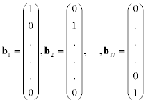
form a standard basis of RN. All other vectors are expressed in terms of the basis bn (n=1, …, N):
The coefficients xn are the components of a vector x and this representation is commonly written in a compact form x=(x1, …, xN)T. The superscript T indicates the transposition that changes column vectors into row vectors and vice versa. The dot product of two vectors x=(x1, …, xN)Tand y=(y1 …, yN)T is
Two vectors x and y are orthogonal if (x, y)=0.
To work with an object, we need some way to measure it. To do so, a vector norm is introduced. A norm of a vector x is a real scalar ![]() x
x![]() with the following properties:
with the following properties:
For a vector x=(x1, …, xN)T, scalar
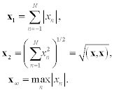
is a norm for any p≥ 1 (the Hölder p-norm). The following norms are commonly used:
Every square matrix generates a linear operator in the Euclidean space RN. If y is a linear function of x, then
The rules for manipulating matrices are those required by the linear mappings. Thus C= A+ B is the sum of two linear functions represented by A and B, where cnm= anm+ bnm. The product AB represents the effect of applying the mapping B, then applying the mapping A. If we have y= A(Bx)=Cx, then components of matrix C are given by the formula
The transposition of A is obtained by reflecting A about its main diagonal:
A diagonal matrix D is all zeros except for dn on the main diagonal: D= diag(d1, …, dN).
Now, let us consider norms of a matrix. Scalar ![]() A
A![]() is a norm of a matrix A if the following conditions are satisfied:
is a norm of a matrix A if the following conditions are satisfied:
The following norms are commonly used:
In what follows the notation ![]() ⋅
⋅ ![]() will denote some norm given above. A matrix norm is consistent with a vector norm if
will denote some norm given above. A matrix norm is consistent with a vector norm if ![]() Ax
Ax![]() ≤
≤ ![]() A
A![]() ⋅
⋅ ![]() x
x![]() . For example,
. For example, ![]() A
A![]() 1 is consistent with
1 is consistent with ![]() x
x![]() 1,
1, ![]() A
A![]() 2 with
2 with ![]() x
x![]() 2, and
2, and ![]() A
A![]() ∞ with
∞ with ![]() x
x![]() ∞.
∞.
The property of matrix definiteness plays an important role in matrix computations. So, a matrix A is positive (negative) definite if (x, A)>0 (< 0) for all nonzero vectors x. If the sign of (x, A) depends on vector x, then matrix A is called indefinite.
In the following, we demonstrate how to calculate the dot product of two vectors.
You could either use the dot function to compute the dot product of two vectors or you could use the dot product operator “.*” and then apply sum to get the dot product. The latter approach is better in performance.
The norm function, as demonstrated below, could be used to find out different norm values of a vector. The second argument determines the order of norm value. In the absence of second argument, the function returns 2-norm. This function also works for a matrix argument in the similar manner.
8.2 Systems of Linear Equations
A system of linear equations may be represented as
where A={anm} is a square matrix of coefficients of size N by N, x =(x1, …, xN)T is a vector of unknowns of size N, and f= (ƒ1, …, fN)T is a known right-hand vector of size N.
There are numerous physical systems which naturally lead to linear equations, for example, the static analysis of structures (bridges, buildings, and aircraft frames) and the design of electrical networks. Many physical systems are modeled by differential equations, which often cannot be solved analytically. As a result, the finite difference approach has to be used to approximate differential equations. This often results in a system of linear equations (if the differential equation is linear) for approximate values of the solution. Also, systems of linear equations may arise as an intermediate stage in other computational processes. Matrix inversion is also an inefficient approach (if we have A− 1, then computation of x is easy: x= A− 1f), because computing an inverse matrix requires about three times as much computation and twice as much storage as does solving a system of linear equations.
To adopt one or another method for the solution of system (8.1) we should take into account properties of matrix A, such as symmetry, definiteness, band structure, and sparsity. This allows us to solve a system of linear equations more efficiently. The adoption of a method also depends on the type of problem under consideration, i.e., whether the problem requires solving a single linear system Ax=f or solving a set of linear equations Axk= fk, k= l, …, M, where matrix A is the same for all k.
The following code listing demonstrates the methods to calculate the inverse and determinate of a matrix. There are two ways to calculate the inverse of a matrix. You could either use the inv function or you could take the reciprocal of the matrix.
8.3 Types of Matrices that arise from Applications and Analysis
8.3.1 Sparse matrices
Matrices with most of the elements equal to zero are called sparse. We can define a matrix A of size N by N as sparse if the number of its nonzero elements ~ N1 + r(γ ≤ 0.5). For example, for N= 103 and γ=0.5, the number of nonzero elements is 31622 (the total number of elements is 106).
8.3.2 Band matrices
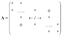
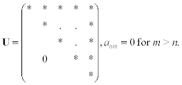
Many applications lead to matrices that are not only sparse, but have a band pattern in their nonzero elements. Matrix A={anm} is called a band matrix if anm= 0 for |n − m| > k where l= 2 k + 1 is the band width:
8.3.3 Symmetric positive definite matrices
Many physical problems lead to symmetric positive definite (SPD) matrices. The properties of SPD matrices follow:
It is rather difficult to determine whether a matrix is positive definite. Fortunately, there are more easily verified criteria for identifying members of this important class. First, all eigenvalues of a positive definite matrix are positive. This can be easily verified with the aid of the Gerschgorin theorem (see Chapter 4). Second, if A is an N by N positive definite matrix, then it has the following properties: (1) anm> 0 for all n; (2) annamm>(anm)2 for n≠ m; and (3) the element of the largest modulus must lie on the leading diagonal.
8.3.4 Triangular matrices
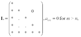
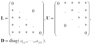
Two types of triangular matrices follow, both of which are easy to work with.
The following function implements the LU decomposition of a tri-diagonal matrix. This utility function finds its application in a number of physical problems.
The application of this function is demonstrated in the following listing.
A system of linear equations Lx= f can be solved by forward substitution:
In an analogous way, a system of linear equations Ux= f can be solved by backward substitution:
The following implementation of forward substitution method is used to solve a system of equations when the coefficient matrix is a lower triangular matrix. The function takes two arguments; the lower triangular coefficient matrix and the right- hand side vector. The output vector is the solution of the systems of equation.
Say, we have the following system of equations given in a matrix form.
Since the coefficient matrix is a lower triangular matrix, forward substitution method could be applied to solve the problem, as shown in the following.
The following implementation of backward substitution method is used to solve a system of equations when the coefficient matrix is an upper triangular matrix. The function takes two arguments; the upper triangular coefficient matrix and the right-hand side vector. The output vector is the solution of the systems of equation.
Say, we have the following system of equations given in a matrix form.
Since the coefficient matrix is an upper triangular matrix, backward substitution method could be applied to solve the problem, as shown in the following.
8.3.5 Orthogonal matrices
If A is an orthogonal matrix, then ATA= I or AT= A− 1, and it is easy to solve linear system (8.1) as x= ATf.
8.3.6 Reducible matrices
A square matrix A is reducible if its rows and columns can be permuted to bring it into the form:
where B is a square matrix of size M by M, D is a square matrix of size L by L, C is a matrix of size M by L, and O is zero matrix of size L by M (M+L=N). This property allows us to break the problem into two smaller ones, usually with a very substantial saving in work. Let us split each of the vectors x and f into two vectors:
8.4 Error Sources
When we solve problem (8.1) by some method, three types of error may occur. First of all, we assume that problem (8.1) is posed exactly. Thus we neglect inevitable errors connected with formulating a problem as a model of scientific process (measurement errors, insufficiently precise basic hypotheses, etc.).
A vector fin (8.1) is not given a priori but must be computed by the data of the exact problem. These computations are performed with a certain error, and instead of f we actually obtain some “perturbed” vector f+ δf. Then instead of problem (8.1) we obtain the “perturbed” problem
We assume this problem is also solvable, and y is the solution. Then
Now the perturbed system (8.4) must be solved. Let us assume that we have some algorithm which produces after a finite number of operations either an exact vector y (if operations are performed error free) or some vector z such, that the error
can be estimated and the error bound can be made arbitrarily small. The quantity ea is called the algorithm error.
In fact any algorithm contains associated floating-point operations, which are connected with errors. These errors amount to the situation that instead of z we obtain some other vector w and the quantity
Finally, instead of the wanted solution x* we compute some vector w. It is natural to take this vector as the approximate solution to problem (8.1) and its error is
8.5 Condition Number
As we discussed before, we have an original problem Ax=f and a perturbed problem A(x+ δx)=f + δf, where δf represents the perturbation in both the right-hand side and A. The objective is to estimate how the uncertainty δf in f is transmitted to δx, that is, to estimate the quantity
It follows from (8.1) and (8.4) that
If we substitute this into the previous expression, we get
is called the standard condition number. This number estimates the maximum magnification of the uncertainty δf. If cond(A) is relatively small, then system (8.1) is well conditioned and δx is relatively small as well. For example, if ![]() δf
δf![]() /
/![]() f
f![]() = 10− 14 and we want
= 10− 14 and we want ![]() δf
δf![]() /
/![]() f
f![]() = 10− 6, then cond(A)=108 is quite acceptable. If cond(A) is relatively large, then we face an ill-conditioned system and we should use some special procedures to obtain an acceptable result.
= 10− 6, then cond(A)=108 is quite acceptable. If cond(A) is relatively large, then we face an ill-conditioned system and we should use some special procedures to obtain an acceptable result.
The direct calculation of the condition number is usually inefficient, as we need to compute an inverse matrix. Therefore, we must resort to estimating the condition number. numEclipse provides the cond function to estimate the condition number as demonstrated in the following code listing.
8.6 Direct Methods
In this part we will consider direct methods. The distinctive feature of these methods is that, ignoring round-off errors, they produce the true solution after a finite number of steps. Let us discuss the basic principles of these methods.
8.6.1 Basic principles of direct methods
The solution is obtained after first factorizing A as a product of triangular matrices, and the form of factorization depends on properties of a matrix A. For general matrices we obtain
where L is a lower triangular matrix with unit diagonal elements, and U is an upper triangular one. For SPD matrices we use the Cholesky factorization
where L is a lower triangular matrix. Hence, a system Ax=f can be transformed into two systems of equations:
The systems are solved simultaneously by forward and backward substitutions, respectively (see (8.2) and (8.3)). The error sources for these methods are the perturbation errors in factors L and U and the rounding errors in solving systems (8.6). An estimation of the work for the LU-factorization yields Nops~ N3, and the Cholesky factorization requires half as much work and storage as the method of LU- factorization.
There is another factorization that is useful. Find an orthogonal matrix Q and upper triangular matrix R so that QAx=Rx=Qf; therefore, x may be obtained by backward substitution on the vector Qf. The attraction of the orthogonal factorization lies in the fact that multiplying A or f by Q does not magnify round-off errors or uncertainties associated with the matrix A or vector f. To see this, note that
since QTQ=I. So the advantage of this approach is that it produces a numerically stable method. However, this method requires twice as much work as the method of LU-factorization. That is why the application of orthogonal transformations to the solution of systems of linear equations is limited to some special cases. As we will see, these transformations have also found application in the eigenvalue problem.
Now we consider the sweep method. This technique is based on a special transformation that can be applied to systems with a band matrix. We restrict ourselves to the case where the matrix of system (8.1) is a tridiagonal one. It is convenient for us to represent a system of equations with a tridiagonal matrix in the explicit form:
The basic idea of the sweep method is to represent a solution in the following form:
which is at least possible for the first equation. Let coefficients αn− 1, and βn − 1, be known, then we can write
After eliminating xn− 1, we rewrite the previous expression as follows:
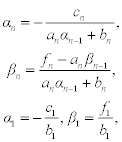
Therefore, coefficients αn and βn are calculated according to the relations
Once the parameters αn and ßn have been computed, we can easily solve system (8.7). To begin with, let us write expression (8.8) for n=N − 1 and the last equation (8.7):
Eliminating xN− 1, we arrive at
All other components xn are calculated using (8.10) for n=N − 1, …, 1. The sweep method is a very efficient technique for solving systems of equations with a tridiagonal matrix because Nops= 8 N − 6.
The following theorem describes conditions which provide stability of the sweep method.
The following function implements the direct method of solving a system of linear equations such that the coefficient matrix is factored into lower- and upper- triangular matrices. The function takes these matrices as arguments along with the right-hand side vector. The implementation is simple and based on the last two implementations of forward and backward substitution. In the first step, forward substitution is applied and then the backward substitution is carried out to find the solution.
We have the following system of equations given in a matrix form.
The following steps show how to apply the direct method to solve this problem.
8.6.2 Error estimation for linear systems
Estimation of the error vector e= x− x* is a delicate task, since we usually have no way of computing this vector. It is possible, at least within the limits of machine precision, to compute the residual vector r= Ax− f, which vanishes if e=o. However, a small residual does not guarantee that the error is small. Let us analyze the relationship between e and r more generally. Observe that r= Ax− Ax*=A(x− x*)=Ae, that is, e= A− 1r. Then the ratio ![]() e
e![]() /
/![]() f
f![]() is
is
But ![]() Ax∗
Ax∗![]() ≤
≤ ![]() A
A![]() ⋅
⋅ ![]() x∗
x∗![]() , so we can replace the denominator on the left side and multiply through by
, so we can replace the denominator on the left side and multiply through by ![]() A
A![]() to obtain the estimate
to obtain the estimate
This inequality asserts that the relative error is small when the relative magnitude of the residual is small and cond(A) is not too large.
8.7 Iterative Methods
Iterative methods for Ax=f are infinite methods and they produce only approximate results. They are easy to define and can be highly efficient. However, a thorough study of the problem is needed in order to choose an appropriate method.
8.7.1 Basic principles of iterative methods
Iterative methods are usually based on the following equivalent form of system (8.1):
where B is an iterative matrix. We construct this form by analogy with (7.1), simply adapting the same principle to system (8.1). The components of the iterative matrix are expressed in terms of the components of matrix A. Vector g is also expressed in terms of matrix A and vector f. It is often not practical to calculate B explicitly but it is implied that in principle this can be done. On the basis of form (8.10), an iterative process is constructed as follows:
Iterative process (8.11) is called stationary and process (8.12) is accordingly called nonstationary. How are iterations x(k) related to the exact answer for problem (8.1)? To clear up this question, let us carry out a simple analysis. Every approximation x(k) may be represented in the following form:
where e(k) is the error vector of kth approximation. After substituting (8.13) into (8.11) and taking into account (8.10), we obtain
then the iterations converge and
There is another sufficient condition that provides convergence: if ![]() B
B![]() < 1, then condition (8.15) is satisfied, because s(B) ≤
< 1, then condition (8.15) is satisfied, because s(B) ≤ ![]() B
B![]() for any matrix norm.
for any matrix norm.
Iterative process (8.13) is connected with the algorithm and rounding errors; the perturbation error does not occur. The algorithm error is easily estimated. For simplicity, the iteration is started with x(0)= g, then
so the smaller the spectral radius of the matrix B, the faster approximations x(k) approach x*. As for the rounding errors, the following estimate may be obtained:
As we can see, iterative methods are very stable in terms of rounding errors.
8.7.2 Jacobi method
Let us represent a matrix A as
Now we can construct an equivalent form (8.10) in the following manner
Therefore, iterative matrix B and vector g for the Jacobi method is
The construction of equivalent form (8.17) consists of solving the nth equation explicitly for the nth unknown and putting everything else on the right-hand side. Because matrix BJ is easily calculated, one can estimate s(BJ) to determine if the Jacobi method is convergent. There are also sufficient conditions which allow for clarifying convergence of the Jacobi method immediately in terms of matrix A. They are: (1) A is a matrix with strong diagonal dominance, so taking into account the structure of Bj, it is easy to show that ![]() BJ
BJ![]() ∞ < 1; and (2) A is an irreducible matrix with weak diagonal dominance.
∞ < 1; and (2) A is an irreducible matrix with weak diagonal dominance.
The implementation of the Jacobi method requires two utility functions, Idu and invdiag. The function Idu decomposes a given matrix into lower triangular, diagonal and upper triangular matrices.
The invdiag function returns the inverse of a given diagonal matrix. It was important to implement as a separate and efficient function rather than using the built-in inv function since the diagonal matrix is sparsely populated and it should not take that much computational effort.
The following code listing implements the Jacobi method using the above utility functions. It takes three input arguments; the coefficient matrix, right-hand side vector and error tolerance.
We have the following system of equations given in a matrix form.
The following steps show how to solve it using the Jacobi method.
It takes 38 iterations to reach the solution with desired accuracy.
8.7.3 Gauss-Seidel method
Let us refer again to representation (8.18). We can construct an equivalent form (8.12) in a different manner:
We do not need to invert the matrices L+ D or U+ D, because we can immediately apply the iteration
The matrix L+D is a lower triangular one and U+D is an upper triangular matrix. Therefore, systems (8.18) and (8.19) are easily solved with respect to x(k+1). Because the explicit calculation of matrix BGS is impractical, the sufficient convergence conditions are of importance. They are: (1) A is a matrix with strong diagonal dominance; (2) A is an irreducible matrix with weak diagonal dominance; and (3) A is a SPD matrix. In this last case, if the Jacobi method converges s(BJ,)< l), then the Gauss-Seidel method has more rapid convergence because s(BGS)=s2(BJ) for this type of matrix.
The following function implements the Gauss-Siedel’s iterative method to solve a system of linear equations. The function signature is same as the Jacobi method.
In the following, we apply the Gauss-Siedel method to the problem in last example.
It shows that the Gauss-Siedel method is superior to the Jacobi method since it takes only 20 iterations to solve the same problem.
8.7.4 Method of relaxation
When employing an iterative method, the main question is how to achieve rapid convergence, or to put this in other words, how to construct an iterative matrix with the smallest s(B) possible. To do this, one should be able to exert control over the properties of iterative matrix B. This can be realized with the use of a special procedure called the method of relaxation.
To begin with, let us discuss the general scheme of this method. Consider system (8.1) with an SPD matrix A. For an arbitrary vector x(k), which is considered as an approximate solution, we define an error function
In order to define another vector x(k+ 1) which differs from x(k) only in the nth component such that φ(x(k + 1)) < φ(x(k)), we put x(k + 1) = x(k) + αbn (bn is the basis vector, see 8.1). Then, it is easy to obtain
where (r(k))n is the nth component of the residual vector: (r(k))n = (Ax(k) − f, bn). The sum of the second and third terms in (8.20) can be made negative; we simply choose so that
where ω is called the relaxation parameter. By choosing parameter a for n= l, …, N we arrive at the following iterative scheme:
The equivalent form (8.10) for this iterative process may be also written as
Now we have an iterative matrix that depends on a parameter ω. One can find such ω that provides the minimal value of s(BJR(ω)). This parameter is called the optimal relaxation parameter and is denoted as ωopt. The method of relaxation (8.21) is based on the Jacobi method (BJR(1) = BJ). It is easy to see that λ(BJR(ω)) = 1 + ω(λ(BJ) − 1). Let − λl ≤ λ(BJ) ≤ λr then the optimal relaxation parameter is
The next logical step is to construct the relaxation method based on the Gauss-Seidel iteration (8.18). Taking into account representation (8.16), one can transform (8.22) into the following equivalent system:
As before, we do not need to invert matrix D+L and the iterative scheme is
Matrix D+ ωL is a lower triangular one, therefore system (8.23) can be easily solved with respect to X(k + 1). It was noticed in practice (in some cases it was proved) that convergence of iterative scheme (8.23) with ω< 1 (under-relaxation) is slower in comparison to ω ≥ 1 (over-relaxation). Thus, ω ≥ 1 is usually used and iterative scheme (8.23) is called the method of successive over-relaxation (SOR). There is only one procedure, proposed by David Young, to calculate the optimal relaxation parameter ω. Let us briefly consider this result.
The Jacobi matrix BJ = I − D− 1 A = − D− 1L − D− 1U is consistently ordered if
for any α≠ 0. For example, block tridiagonal matrices of the form
where Dm is a square matrix of size Nm × Nm(m = 1, …, p), Lm and Um-1 are matrices of size Nm × Nm + 1 and Nm + 1 × Nm respectively (m = 2, …, p; N1 + … + Np = N) are consistently ordered. Let A be an SPD consistently ordered matrix. If the Jacobi method converges (s(BJ)<1), then the optimal relaxation parameter for the SOR is calculated by the formula:
Calculating the spectral radius of the Jacobi matrix BJ requires an impractical amount of computation, so this is seldom done. However, relatively inexpensive rough estimates of s(BJ) can yield reasonable estimates for the optimal value of ωopt.
As for other types of matrices, we do not know how to determine the optimal relaxation parameter. However, there are some conditions which are sufficient for the convergence of the SOR. First, if A is an SPD matrix, then the SOR converges when 0 < ω< 2. In this case the relaxation parameter given by (8.24) is still close to optimal, because ωopt − 1 ≤ s(BSOR) ≤ (ωopt − 1)1/2. Second, if A is a matrix with strong diagonal dominance, or with weak diagonal dominance and irreducible, then some *>1 exists. The SOR converges when 0 < ω<ω*.
Successive Over Relaxation or SOR method introduces a parameter to control the convergence of the iterative process, as shown in the following implementation. The signature of following function is same as previous functions except the addition of w control parameter.
We apply the SOR method to the same problem discussed in previous sections. There are a number of methods to find the optimal value of control parameter, w. For the sake of simplicity, we have arbitrarily chosen the value in the following.
Readers are encouraged to try different values to see how it impacts the convergence speed.
It takes only 9 iterations to solve the same problem which shows that SOR is the best iterative method to solve a system of linear equations.
8.7.5 Variational iterative methods
It is evident from the foregoing account that, in general, we need some information about the spectral radius of an iterative matrix in order to analyze convergence of an iterative method. Often, it is impractical to calculate or estimate s(B). There are methods wherein convergence is ensured by special parameters, which in turn depend on an approximate solution. It is clear that the realization of such methods gives rise to non-stationary iterative processes (8.12).
We shall consider an iterative scheme of the following form:
where τk ≠ 0 is an iterative parameter. Let us introduce residual r(k) = Ax(k) − f. Using (8.25), the residual vector r(k+ 1) associated with the next approximation can be expressed in terms of r(k)
Thus, we can determine parameter τk ≠ 0 in such a manner that ![]() r(k + 1)
r(k + 1)![]() 2 will be minimal. The norm of residual r(k+ 1) is expressed as follows:
2 will be minimal. The norm of residual r(k+ 1) is expressed as follows:
Condition φ′(τk) is the condition of the minimum of φ(τk), because
Iterative schemes (8.25) and (8.27) together comprise the method of minimal residual. Let us analyze convergence of this method. If we substitute (8.27) into (8.26), then
Both terms in the right-hand side of (8.28) are positive, therefore
for any definite matrix A and this proves convergence of iterative scheme (8.25). Now consider the rate of convergence of the method of minimal residual. Suppose a matrix A of system (8.1) has the following properties:
If all eigenvalues of matrix A are real, then we can put
For SPD matrices one can use iterative scheme (8.25) and calculate τk by other means. Instead of the residual, let us consider the actual error e(k)= x(k)− x*. Taking into account that Ax*=f, from (8.25) we obtain
We have no way of calculating the actual error, but
So we can determine τk by minimizing the value of (e(k + 1), Ae(k + 1)). Using (8.29) we obtain
Condition φ′(τk) = 0 is the condition of the minimum of φ(τk), because φ″(τk) = (r(k), Ar(k)) > 0, (A is an SPD matrix). So τk is determined as follows:
Iterative scheme (8.25) with τk from (8.30) is called the method of steepest descent. Properties of this method are similar to the method of minimal residual.
On the basis of the method of steepest descent we can construct an iterative method with more rapid convergence. Let us modify (8.25) and write it in the following form:
Here d(k) is a direction vector which points towards the solution of a linear system. In the method of steepest descent, direction vectors are residuals r(k), but this choice of directions turns out to be a poor one for many systems. It is possible to choose better directions by computing direction vectors as
Parameters ak are determined in such a way as to provide orthogonality of vectors d(k) and Ad(k − 1)((d(k), Ad(k − 1)) = 0), then
Using the same considerations as those for the method of steepest descent, rk is determined so that it provides a minimal value of (e(k + 1), Ae(k + 1)). Then we have
Iterative scheme (8.31) with equations (8.32), (8.33), and (8.34) comprise the conjugate gradient method. The error of the kth approximation generated by this method obeys the following bound
The distinctive feature of this method is that, ignoring round-off errors, we obtain r(k)= 0 at some k≤ N, therefore x(k)= x*. By this means we need no more than N iterations to achieve the true solution. For large systems of equations this is not such a promising result. Nevertheless, in some cases the conjugate gradient method and its modifications produce very rapid convergence.
8.8 Exercises
The problems consist of two parts:
1) solve a system of linear equations using LU-factorization (systems 1–20),
2) solve a system of linear equations using Gauss-Seidel method (systems 21–30).
Estimate the error of approximate solution. Methodical comments: to compute the LU-factorization use the function [L,U] = ludecomp (A) ; to estimate the condition number use the function cond (A).


