
Appendix 6.1: Matrix Operations
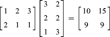
In general, think of two matrices, A and B, and their (inner) product C:
![]()
The first element in the inner product ![]() is the product of the first row of A and the first column of B, that is,
is the product of the first row of A and the first column of B, that is, ![]()
![]() . Similarly,
. Similarly, ![]() is the inner product of the first row of A and the second column of B. C is the collection of inner products of the rows of A and the columns of B. Verify this for yourselves.
is the inner product of the first row of A and the second column of B. C is the collection of inner products of the rows of A and the columns of B. Verify this for yourselves.
Excel requires that we know the dimension of C before we ask Excel to calculate the inner product. We first highlight a ![]() set of cells (do not press Enter yet). Type the command = mmult(A,B) and then simultaneously press CTRL-SHIFT-ENTER.
set of cells (do not press Enter yet). Type the command = mmult(A,B) and then simultaneously press CTRL-SHIFT-ENTER.
You can also get the inverse of a matrix. It must be a square matrix. Take matrix C as an example. Its inverse is (a full discussion of this operation is given next):
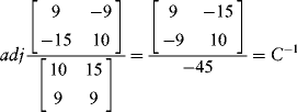
The denominator (–45) is the determinant of C. If this value is zero, then the inverse is undefined.
The Excel sequence that computes a matrix inverse again requires that we know the dimensions. We highlight a ![]() set of cells once again and then type the command = minverse(C), followed by the CTRL-SHIFT-ENTER sequence.
set of cells once again and then type the command = minverse(C), followed by the CTRL-SHIFT-ENTER sequence.
I want to show you a more meaningful multivariate regression application. Let Y be a set of N observations (for example, the returns to N stocks for the current month). Let X be a ![]() matrix of regressors, including the column of ones associated with the intercept. The regressors can be thought of as factors like earnings growth, earnings surprises, firm size, and so on, that returns depend upon. Let β be a
matrix of regressors, including the column of ones associated with the intercept. The regressors can be thought of as factors like earnings growth, earnings surprises, firm size, and so on, that returns depend upon. Let β be a ![]() column vector of parameters that we wish to estimate and let ε be a
column vector of parameters that we wish to estimate and let ε be a ![]() column vector of disturbances. Let's write our model as follows. (From now on, we will denote the dimension of β as k × 1, understanding that k includes the intercept.)
column vector of disturbances. Let's write our model as follows. (From now on, we will denote the dimension of β as k × 1, understanding that k includes the intercept.)
![]()
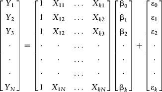
This is how we visualize our data and our simple linear model. The usual assumptions apply (the errors are independent and identically distributed [IID], meaning zero with constant variance and uncorrelated with the regressors). If we want to make inferences and test hypotheses, we add the assumption that the errors are ![]() , understanding that the population variance is unknown and must consequently be estimated. Tests and inferences proceed under the t-distribution with degrees of freedom
, understanding that the population variance is unknown and must consequently be estimated. Tests and inferences proceed under the t-distribution with degrees of freedom ![]() .
.
We wish to estimate the ![]() vector β. I will do this now. First, write the model in matrix
vector β. I will do this now. First, write the model in matrix
![]()
Note that ![]() and
and ![]() times
times ![]() , which by the rules of matrix algebra is conformable for multiplication, that is,
, which by the rules of matrix algebra is conformable for multiplication, that is, ![]() . Finally,
. Finally, ![]() .
.
The inner product (Xβ) is the product of a ![]() matrix X and a
matrix X and a ![]() matrix of parameters β, which has dimension
matrix of parameters β, which has dimension ![]() (a column vector). As before, the first element in Xβ is the product of the first row in X and the vector β, the second element in the second row in X and the vector β, and so forth.
(a column vector). As before, the first element in Xβ is the product of the first row in X and the vector β, the second element in the second row in X and the vector β, and so forth.
Now, multiply both sides by the transpose of X, which we call ![]() . If
. If ![]() , then
, then ![]() . Our model now looks like this:
. Our model now looks like this:
![]()
![]() has dimensions
has dimensions ![]() ,
, ![]() is
is ![]() , and therefore
, and therefore ![]() is
is ![]() , and finally
, and finally ![]() is
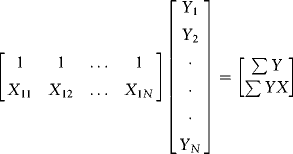
is ![]() . In Excel, highlight a
. In Excel, highlight a ![]() column of cells (do not press Enter) and follow this with the command =mmult(transpose(X),Y) and simultaneously press CTRL-SHIFT-ENTER.
column of cells (do not press Enter) and follow this with the command =mmult(transpose(X),Y) and simultaneously press CTRL-SHIFT-ENTER.
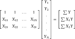
Let's now solve this system for β. First, eliminate X′ε. Since the regressors are assumed independent of the errors, then this term is zero, anyway (specifically, its expectation is zero). Now, we are looking at the system:
![]()
To do this, we must eliminate ![]() (the square matrix) by dividing both sides by
(the square matrix) by dividing both sides by ![]() , that is, we multiply by its inverse
, that is, we multiply by its inverse ![]() . Let's do that now.
. Let's do that now.
![]()
![]()
The statistic b is the least squares estimate of population parameter β. Here's how we would do this in Excel. First, we use Excel's naming convention by highlighting vectors and matrices, and giving them names. Alternatively, in Excel, click on Formulas and select appropriately among the Name Manager (you can change and delete names) and Define Name for new arrays. Let's highlight the ![]() matrix we solved for earlier and in the top left command window, name is
matrix we solved for earlier and in the top left command window, name is ![]() . Likewise, highlight the vector
. Likewise, highlight the vector ![]() and name it
and name it ![]() . To estimate β, highlight a
. To estimate β, highlight a ![]() column of cells. Then type the command, = mmult(XX,XY) followed by CTRL-SHIFT-ENTER.
column of cells. Then type the command, = mmult(XX,XY) followed by CTRL-SHIFT-ENTER.
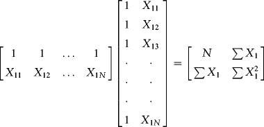
This is what we need to know in Excel. But it seems to be a waste to stop here when we could use this framework to get a deeper understanding of the algebra of least squares (we will be doing a lot of regression in this book). Let's follow up with a simpler illustration, using a single regressor. What does ![]() look like? How about
look like? How about ![]() ? The first is a cross-product matrix. For the case with a single regressor and an intercept,
? The first is a cross-product matrix. For the case with a single regressor and an intercept, ![]() is:
is:
The matrix ![]() is the inner product of the regressors (this is a quadratic form just like
is the inner product of the regressors (this is a quadratic form just like ![]() in a bivariate regression). We build
in a bivariate regression). We build ![]() as follows:
as follows:
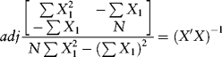
What is the inverse of ![]() ? It is the adjoint matrix of
? It is the adjoint matrix of ![]() divided by the determinant of
divided by the determinant of ![]() . The determinant is:
. The determinant is:
![]()
The inverse is then the adjoint of ![]() given in the numerator in the following equation, divided by the determinant, that is, it is a
given in the numerator in the following equation, divided by the determinant, that is, it is a ![]() matrix
matrix ![]() .
.
We can generalize to the two-regressor case. You can see how the dimensionality of the problem increases. Here is the ![]() matrix:
matrix:
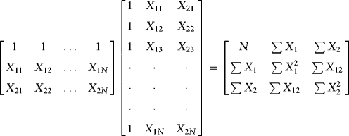
The ![]() matrix is therefore:
matrix is therefore:
We multiply this by the inverse of ![]() to get the least squares estimate of β.
to get the least squares estimate of β.
It is convenient that Excel has regression commands like slope, linest, and trend that do the algebra for us. In many cases, however, such as for portfolio optimization, we must do the dirty work ourselves. Fortunately, it is not too difficult and the process itself gives us deeper insight into the optimization problem.