
Appendix 10.1: Active Space
For active portfolios consisting of many benchmarks, it is often convenient to compress the various benchmarks into a single composite benchmark. That way, we compare k active portfolios to a single benchmark. It not only reduces the dimensionality of the problem from 2k × 2k to a (k + 1) × (k + 1) problem, but simplifies computations and interpretations of active risk. What we need to do, therefore, is to somehow aggregate the benchmarks into a single overall benchmark and compare all the active holdings to this single benchmark. Admittedly, that is not intuitive, but we can hope that it will make more sense after I develop the concept for you.
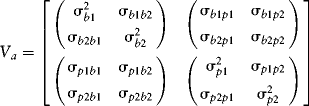
First, I construct a special matrix that will aggregate the benchmark variances and covariances into a single row and column. For the two-asset case it looks like this:

Recall Va:
Aggregating the benchmarks is accomplished by m′Vam, which reduces to:
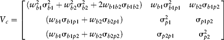
Thus, where we started with a 2k × 2k active covariance matrix, we now work with a matrix of dimension k + 1, in which the first row and column summarize the covariances between the benchmarks and portfolios (or assets). The 2 × 2 diagonal submatrix in the lower right section summarizes the risks associated with the actively managed portfolio positions. This setup generalizes to any given 2k × 2k active covariance matrix. That is, the combined active covariance matrix Vc will consist of a k × k covariance matrix for the actively managed assets bordered by a single row and column summarizing the benchmark and actively managed covariances.
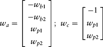
Likewise, we similarly compress the active weight vector such that the first element in the combined weight vector simply represents the short position in the benchmark.
It is not difficult to prove the following equivalency:
![]()