
Chapter 9
Telecommunication Pricing: Smart Versus Dumb Pipes*
ATANU LAHIRI
9.1 Introduction
Discriminatory pricing of telecommunication services today is reminiscent of practices that date back to the eighteenth century, when navigation tolls varied from one cargo type to another—the toll for a ton of sand was not the same as that for a ton of timber [3]. Similarly, consumers of wireless services are now paying different per-byte prices for traffic generated by different services, such as voice calls, SMS (short message service) text messages, picture mails, and mobile Internet [2]. For instance, if one assumes a data rate of 100 KB/min of voice, and 100 bytes per SMS text, a price of ![]() cents/min of voice turns out to be equivalent to $1/MB, whereas a price of 20 cents per SMS text amounts to a whopping $2000/MB [1].
cents/min of voice turns out to be equivalent to $1/MB, whereas a price of 20 cents per SMS text amounts to a whopping $2000/MB [1].
Such discriminatory pricing, particularly the pricing of text messages, has recently come under tremendous opposition from consumers—to the extent that even the US Senate felt compelled to examine its legality and economic impacts [4]. Experts testifying at a hearing at the US Senate Judiciary Committee argued that the average price of an SMS text message far exceeded the marginal cost of the wireless path [5], with no apparent economic justifications. Even the Wall Street Journal, which is known for its dislike for regulations on corporations, voiced opposition to such pricing, demanding a system where all bytes would be treated as just bytes. Mossberg [6], in his weekly column there,
“We need a wireless mobile device ecosystem that mirrors the PC/Internet ecosystem, one where the consumers' purchase of network capacity is separate from their purchase of the hardware and software they use on that network. It will take government action, or some disruptive technology or business innovation, to get us there.”
Carriers, on the other hand, have been vocal at the Senate hearing about their support for discriminatory pricing. Some carriers even took additional steps towards protecting their smart-pipe strategy; for instance, fearing that open platforms such as Android—along with its user-developed services that could not be tagged or metered separately—will disrupt discriminatory pricing, AT&T stayed away from them until 2010 [7].
The common wisdom is thus that dumb pipes work in favor of consumers and smart pipes in favor of carriers. In this chapter, we put this wisdom to economic tests. We will do so by comparing the two pricing regimes in terms of their impacts on profits and welfare. In economic terms, the smart-pipe strategy means pricing different services differently. For example, consider the following pricing by a national carrier: for voice calls, one can either choose a plan that costs $80 a month and includes 1000 min of call time or another that costs $60 a month but includes only 700 min. Consumers can also purchase 300 text messages for a price of $5 a month, or 1000 text messages for $10 a month. Likewise, they can get limited access to the web for $10 a month, or unlimited access for $15 a month. For each service, consumers thus pick from a separate menu of plans.
In the case of dumb pipes, however, a carrier would simply price the traffic carried, giving each consumer the right to allocate the purchased traffic between various services according to his/her preferences. Thus, there is just one menu to choose from. The dumb-pipe strategy is best characterized as quasi-bundling [8]—it is a way of bundling several services into one common bundle, namely, “bytes,” while leaving to each consumer the task of determining his/her actual bundle composition. An astute reader may immediately contrast this with conventional bundling that puts the seller in charge of deciding the bundle composition [9]. We develop a two-stage model of quasi-bundling in this chapter.
We will model the monopolist's tariff design problem assuming that it faces a heterogeneous market. The monopoly setting is relevant to telecommunications. Although the wireless market in the United States has several major players, each happens to possess substantial monopoly power. This is reflected in the fact that the price charged for carrying a text message is often several hundred times the marginal cost of carrying it. The close relationship of a carrier with handset manufacturers, along with various other consumer lock-in mechanisms, contributes to such pricing power. Further, while modeling the monopoly problem, we will ignore all over-limit usage and revenues resulting from such usage; over-limit usage occurs when, for example, a consumer who is on a 1000-min plan uses 1100 min in a month. As explained by Masuda and Whang [10], this simplification is reasonable when a consumer's monthly usage is deterministic.
For the purpose of exposition, we will only consider settings in which the monopolist faces discrete consumer types and sells multiple services. When it sells smart pipes, it offers a separate price schedule (or menu) for each service. Each schedule consists of a number of plans, one aimed at each consumer type, and each plan provides a fixed amount of usage for a price. On the other hand, when thecarrier sells dumb pipes, it faces the task of designing only one price schedule to price traffic consumption; each plan then provides a certain level of traffic usage for a price.
We will examine two models, each with two types of consumers. In the first model, consumers differ primarily in their incomes and those with higher incomes are willing to pay more for every service. In other words, consumer preferences are uniformly ordered across services. In the second one, this ordering is not uniform, just as one would expect when preferences are driven primarily by consumers’ idiosyncratic tastes: one segment of consumers is willing to pay more for certain services and the other segment is willing to do the same for the rest.
For the two models mentioned earlier, uniform ordering and nonuniform ordering, we will compare all three surpluses—producer, consumer, and social—under smart pipes with that under dumb pipes. We will show that the prevalent view regarding the welfare impacts of smart and dumb pipes hold in certain circumstances, but it does not in many others. In particular, we will identify circumstances in which smart pipes surprisingly lead to a higher consumer surplus. A related finding is that smart pipes can lead to a higher social surplus. Finally, we will discuss why the wisdom that smart pipes increase profits may not hold when consumer types are ordered nonuniformly.
9.2 Uniform Ordering
Consider a carrier serving a market with two types of consumers, indistinguishable ex ante to the carrier. Let the consumer types be indexed by i, ![]() or 2. Types 1 and 2 comprise fractions
or 2. Types 1 and 2 comprise fractions ![]() and f, respectively, of the whole population. The firm offers n different wireless services, which are indexed by j,
and f, respectively, of the whole population. The firm offers n different wireless services, which are indexed by j, ![]() .
.
The value of a service to a consumer is taken to be of the form ![]() , where
, where ![]() is a constant, t is the amount of the service used (in bytes), and
is a constant, t is the amount of the service used (in bytes), and ![]() . Value functions of this form have the support of empiricists [11]. Besides, they have desirable properties—they are concave and also exhibit constant relative risk aversion [12]. In our context, the parameter
. Value functions of this form have the support of empiricists [11]. Besides, they have desirable properties—they are concave and also exhibit constant relative risk aversion [12]. In our context, the parameter ![]() reflects the desire for diversity in use of services: a consumer with a higher
reflects the desire for diversity in use of services: a consumer with a higher ![]() prefers allocating traffic more evenly between various services than does a consumer with a lower
prefers allocating traffic more evenly between various services than does a consumer with a lower ![]() . Following the paper on bundling by Armstrong [13], we will assume hereafter that the total value of a set of services to a consumer is the sum of their individual values:
. Following the paper on bundling by Armstrong [13], we will assume hereafter that the total value of a set of services to a consumer is the sum of their individual values:
When the consumer types are uniformly ordered, we can assume without loss of generality that ![]() ,
, ![]() . Thus, one consumer type, namely, type 2, gets an equal or higher value from every service vis-á-vis the other, namely, type 1. Such a scenario is expected when type 2 has a substantially higher income vis-á-vis type 1 and, therefore, is willing to pay more for every telecommunication service. In the next section, we will examine the other scenario, in which consumer type 2 gets higher values from some services, but consumer type 1 gets so from the rest.
. Thus, one consumer type, namely, type 2, gets an equal or higher value from every service vis-á-vis the other, namely, type 1. Such a scenario is expected when type 2 has a substantially higher income vis-á-vis type 1 and, therefore, is willing to pay more for every telecommunication service. In the next section, we will examine the other scenario, in which consumer type 2 gets higher values from some services, but consumer type 1 gets so from the rest.
For the sake of clarity, we will assume a constant marginal cost throughout our analysis. We will also normalize all fixed costs to zero as they are sunk for our purposes.
The firm (i.e., the carrier) offers nonlinear price schedules consisting of plans of the form ![]() , where p is the price charged for t bytes of usage. If the carrier employs the smart-pipe strategy, it announces a separate price schedule for each service. When using the dumb-pipe approach, it announces just one price schedule to price the total traffic consumption (see Fig. 9.1).
, where p is the price charged for t bytes of usage. If the carrier employs the smart-pipe strategy, it announces a separate price schedule for each service. When using the dumb-pipe approach, it announces just one price schedule to price the total traffic consumption (see Fig. 9.1).

Figure 9.1 Timeline.
9.2.1 Dumb Pipe
In the case of dumb pipes, the carrier offers a single schedule to price traffic. The price schedule or menu consists of two plans here, (![]() ,
, ![]() ) and (
) and (![]() ,
, ![]() ), aimed at types 1 and 2, respectively. A consumer who purchases a plan has to decide on how much to use for each service. For a type-i consumer, this allocation problem—assuming that the consumer is allocating t bytes of traffic—is as follows:
), aimed at types 1 and 2, respectively. A consumer who purchases a plan has to decide on how much to use for each service. For a type-i consumer, this allocation problem—assuming that the consumer is allocating t bytes of traffic—is as follows:

Let the solution to the above problem be (![]() ), that is,
), that is, ![]() is the traffic that a type-i consumer will allocate to service j when dividing t units of traffic optimally between the n services. This solution can be found from
is the traffic that a type-i consumer will allocate to service j when dividing t units of traffic optimally between the n services. This solution can be found from

Equation (9.1 ) is readily solved for the value functions described in Assumption 9.2. For type-1 consumers, they are equivalent to the following equations.

The solution for type-1 consumers is, therefore,

Figure 9.2, which assumes a two-service scenario, shows the fractions of total traffic that a type-1 consumer allocates to the two services.

Figure 9.2 Type-1 consumer's traffic allocation for  and
and  .
.
When ![]() is small, each consumer allocates a greater percentage to the service that he/she values more, which is the service with the higher
is small, each consumer allocates a greater percentage to the service that he/she values more, which is the service with the higher ![]() parameter—service 1 in the example. When
parameter—service 1 in the example. When ![]() is large, his/her allocation becomes more even. Clearly,
is large, his/her allocation becomes more even. Clearly, ![]() reflects his/her affinity for diversity in use of services.
reflects his/her affinity for diversity in use of services.
For type-2 consumers, Eq. (9.1 ) can be rewritten as

The solution for type-2 consumers is, therefore, similar.

We can derive the maximum value or the reservation price for traffic of each consumer type by substituting the optimal ![]() values back into the respective value functions. Let
values back into the respective value functions. Let ![]() denote the maximum value that a consumer of type i can derive from optimally allocating t units of traffic to different services. Then
denote the maximum value that a consumer of type i can derive from optimally allocating t units of traffic to different services. Then

We now turn to the problem of designing a pricing menu consisting of two plans, namely, (![]() ,
, ![]() ) and (
) and (![]() ,
, ![]() ). Although this appears difficult at first sight, comparing Eq. (9.6 ) with Assumption 9.2, we can easily see that the problem of designing a menu for traffic is, in fact, structurally no different from the problem of pricing any one service. Further,
). Although this appears difficult at first sight, comparing Eq. (9.6 ) with Assumption 9.2, we can easily see that the problem of designing a menu for traffic is, in fact, structurally no different from the problem of pricing any one service. Further, ![]() ,
, ![]() , implies that
, implies that ![]() , which, in turn, means that type 2 is also the high type here just as it is in the case of any service.
, which, in turn, means that type 2 is also the high type here just as it is in the case of any service.
- Individual Rationality. A consumer will only purchase a plan that offershim/her a nonnegative utility. The individual rationality constraints for types 1 and 2 are
IR.1
 IR.2
IR.2
- Incentive Compatibility. Each consumer picks the plan that generates the highest surplus for him/her. These constraints are
IC.1
 IC.2
IC.2
The carrier's problem is to maximize the profit subject to the individual rationality and incentive compatibility constraints above. Its profit, with the plans selected as posited, is
There are three possible outcomes [14]: no one is served, only high type consumers are served, or all are served. When only the high type (type 2) is served, the firm extracts the entire surplus—the price equals the reservation price of the high type. When both types are served, the carrier's profit is maximized when the low type is indifferent between purchasing and not purchasing, and the high type, between purchasing the plan aimed at the low type and its own plan. Hence, only the IR1 and IC2 constraints are binding. Using the IR1 and IC2 constraints to substitute for ![]() in terms of
in terms of ![]() ,
, ![]() , we can immediately reduce the firm's problem to
, we can immediately reduce the firm's problem to
Henceforth, we will refer to the optimal schedule—the solution to the second-degree discrimination problem—by ![]() (
(![]() ,
,![]() ), (
), (![]() ,
,![]() )
)![]() . The optimal usages, along with the corresponding optimal profit and the consumer surplus for each consumer type, are shown in Table 9.1.
. The optimal usages, along with the corresponding optimal profit and the consumer surplus for each consumer type, are shown in Table 9.1.
The optimal prices can easily be obtained from the optimal usages and the fact that IR1 and IC2 become equalities.
As a benchmark, the table also provides the first-best (FB) solution, the one the carrier would use when it can identify each consumer's type and accordingly charge each a different price. Let us first compare usages for each consumer type. The usage of traffic by the high type (type 2) is unaffected by the degree of discrimination—it is always at a level where its marginal willingness to pay equals the marginal cost. The same is not the case for the low type (type 1). If low type consumers make up a small fraction of the population, that is, ![]() , the carrier will not serve them at all. Even when the carrier serves them, it only serves them a quantity that is below the FBlevel.
, the carrier will not serve them at all. Even when the carrier serves them, it only serves them a quantity that is below the FBlevel.
9.2.2 Smart Pipe
When using the smart-pipe strategy, the carrier offers a separate schedule for each of the n services. The schedule for a service j consists of two plans, ![]() (
(![]() ,
,![]() ), (
), (![]() ,
,![]() )
)![]() , one for each of the two consumer types. Note that this problem is separable across services—the firm can independently find the optimal nonlinear price schedule for each service. When
, one for each of the two consumer types. Note that this problem is separable across services—the firm can independently find the optimal nonlinear price schedule for each service. When ![]() , the solution for service j will be the same as the one in Table 9.1, except that
, the solution for service j will be the same as the one in Table 9.1, except that ![]() and
and ![]() will need to be replaced by
will need to be replaced by ![]() and
and ![]() , respectively. Henceforth, we are going to denote this optimal schedule for service j by
, respectively. Henceforth, we are going to denote this optimal schedule for service j by ![]() (
(![]() ,
,![]() ), (
), (![]() ,
,![]() )
)![]() .
.
Table 9.1 Optimal Menu for Pricing Traffic; ![]()
| Case | Usage | Profit | Consumer Surplus |
| First-Degree Discrimination | |||
 |
0 | ||
| all served |  |
0 | |
| Second-Degree Discrimination | |||
 |
0 | ||
| all served |  |
 |
|
| 0 | |||
| type 2 served | 0 |
9.2.3 Smart Pipe Versus Dumb Pipe
Without the loss of generality, we can assume that ![]() so that
so that ![]() . This ordering also implies that
. This ordering also implies that ![]() . When not all
. When not all ![]() parameters are equal,1 the two pricing strategies or regimes are equivalent only if the proportion of the high type is at an extreme level, for example, when
parameters are equal,1 the two pricing strategies or regimes are equivalent only if the proportion of the high type is at an extreme level, for example, when ![]() . When
. When ![]() , under either regime only type-2 consumers are served and their usage is at a level where the marginal cost equals the marginal value. However, significant differences between the two pricing regimes exist at all other values of f. For example, when
, under either regime only type-2 consumers are served and their usage is at a level where the marginal cost equals the marginal value. However, significant differences between the two pricing regimes exist at all other values of f. For example, when ![]() , all consumers use all services regardless of the regime but their usage amounts differ; as a result, profits and consumer surpluses differ. When
, all consumers use all services regardless of the regime but their usage amounts differ; as a result, profits and consumer surpluses differ. When ![]() , the smart-pipe strategy restricts certain services to type-2 consumers, while the dumb-pipe strategy makes all services available to all consumers. When
, the smart-pipe strategy restricts certain services to type-2 consumers, while the dumb-pipe strategy makes all services available to all consumers. When ![]() , type-1 consumers are not served at all in the case of dumb pipes; however, in the case of smart pipes, they are served all services whose
, type-1 consumers are not served at all in the case of dumb pipes; however, in the case of smart pipes, they are served all services whose ![]() parameters are strictly less than
parameters are strictly less than ![]() .
.
One of the fascinating consequences of Theorem 9.1 is that the consumer surplus can be higher under smart pipes. To see this clearly, consider the scenario in which the monopolist sells two services, namely, 1 and 2, with ![]() . Depending on the value of f, the fraction of high type consumers, the equilibrium usages obtained from Table 9.1 is going to be in one of the four distinct regions, labeled U1, U2, U3, and U4 in Figure 9.3, with different equilibrium outcomes. In U1, where
. Depending on the value of f, the fraction of high type consumers, the equilibrium usages obtained from Table 9.1 is going to be in one of the four distinct regions, labeled U1, U2, U3, and U4 in Figure 9.3, with different equilibrium outcomes. In U1, where ![]() , both types enjoy both services irrespective of the pricing strategy. However, in U2, where
, both types enjoy both services irrespective of the pricing strategy. However, in U2, where ![]() , type 1 can no longer enjoy service 2 under smart pipes, but it still enjoys both services under dumb pipes. Moving on to U3, where
, type 1 can no longer enjoy service 2 under smart pipes, but it still enjoys both services under dumb pipes. Moving on to U3, where ![]() , type 1 continues to enjoy service 1 if the carrier employs the smart-pipe strategy, although it gets fully shut out if the carrier implements dumb pipes. Finally, type 1 is fullyshut out in U4, where
, type 1 continues to enjoy service 1 if the carrier employs the smart-pipe strategy, although it gets fully shut out if the carrier implements dumb pipes. Finally, type 1 is fullyshut out in U4, where ![]() , regardless of the pricing strategy. Note that type 2, being the high type, enjoys all services in all regions.
, regardless of the pricing strategy. Note that type 2, being the high type, enjoys all services in all regions.

Figure 9.3 Consumer surplus comparison with uniformly ordered consumer types; smart pipe (solid) versus dumb pipe (dashed);  ,
,  ,
,  ,
,  ,
,  , and
, and  .
.
Figure 9.3 also depicts how the consumer surplus varies with the fraction of type-2 consumers across these regions. In region U3, the dumb-pipe strategy shuts out the low type consumer, driving the consumer surplus to zero, but smart pipes still allow the low type to use one of the two services, leading to a strictly positive consumer surplus. More intriguingly, in parts of region U2, where both types are served both services under dumb pipes, smart pipes lead to a higher consumer surplus despite restricting the low type to only one service.
Let us now examine the intuition behind these apparently counterintuitive results. As expected, the dumb-pipe approach favorably affects the consumer surplus in U1, and in parts of U2, because it lets all consumers freely allocate the purchased traffic between the two services. However, in U3 and in parts of U2, such pricing significantly reduces the carrier's incentive to serve the low type. Because the carrier is not able to restrict the low type to only one service in these regions, serving the low type adequately there requires ceding too large an information rent (i.e., surplus) to the high type. On the other hand, the smart-pipe strategy allows the carrier to restrict service 2 to the high type, creating more flexibilities to curb the information rent. Viewed differently, when restricting one service to only one consumer type is no longer an option, the carrier is forced to severely underserve the low type in order to control the consumer surplus that goes to the high type. The net implication is that the prevalent view held by consumers against smart pipes becomes inapplicable when the fraction of the high type is moderate to large.
Let us now consider the impact of ![]() . Figure 9.4 illustrates how
. Figure 9.4 illustrates how ![]() changes with
changes with ![]() . Evidently,
. Evidently, ![]() is lower at lower values of
is lower at lower values of ![]() , that is, consumers find smart pipes preferable over a wider range of values of f.
, that is, consumers find smart pipes preferable over a wider range of values of f.

Figure 9.4  versus
  ;
;  ,
,  ,
,  ,
,  , and
, and  .
.
This phenomenon can be explained as follows. Recall that ![]() indicates consumers’ desire for diversity in their use of services. When
indicates consumers’ desire for diversity in their use of services. When ![]() is close to 1, consumers want to allocate traffic more evenly between services. On the other hand, when
is close to 1, consumers want to allocate traffic more evenly between services. On the other hand, when ![]() is close to 0, consumers benefit more by concentrating their usage on a few services. Hence, the primary benefit of dumb pipes—the freedom to allocate traffic between services—is less valuable to consumers at lower values of
is close to 0, consumers benefit more by concentrating their usage on a few services. Hence, the primary benefit of dumb pipes—the freedom to allocate traffic between services—is less valuable to consumers at lower values of ![]() .
.
We now turn to a comparison of the social surpluses. According to Lemma 9.4, when consumers are uniformly ordered, the smart-pipe strategy is superior from the carrier's viewpoint. More interestingly, it suggests that smart pipes accomplish a higher producer surplus even in regions in which it leads to a higher consumer surplus. Therefore, in contrast to what consumer advocates believe, the smart-pipe strategy is not a mechanism that merely transfers surplus from consumers to the carrier. As indicated by the numerical example in Figure 9.5, discrimination can also lead to a higher social surplus.

Figure 9.5 Social surplus comparison with uniformly ordered consumer types; smart pipe (solid) versus dumb pipe (dashed);  ,
,  ,
,  ,
,  ,
,  , and
, and  .
.
We now formally state the comparison of the social surpluses under the two strategies as our next theorem.
The implication is obvious. If we impose a ban on the smart-pipe strategy, it can quickly become a lose–lose proposition for both the carrier and consumers. Only in U1, which is characterized by a few high income consumers and a large number of low income consumers, the ban would work as expected, that is, it would lead to a higher consumer surplus as well as a higher profit.
The existing literature on second-degree price discrimination also identifies instances in which discrimination is preferable (to uniform pricing across consumer classes) from the social planner's viewpoint [15–17]. Similarly, the literature on third-degree discrimination also finds instances in which the discrimination across different consumer markets leads to a higher social surplus [18, 19]. In essence, we are here examining discrimination across services (calling, messaging, etc.) that use the same resource (traffic). Despite the difference in the nature of discrimination, the intuition behind Theorem 9.5 is still very similar to what one finds in the existing literature: when discrimination is not possible, the producer feels constrained; in response, it reduces its output and forgoes certain consumer segments, which, in turn, adversely affects social welfare. Clearly, our finding here has significant policy implications for governments that are currently debating how to regulate the telecommunication sector optimally from the societal perspective.
9.3 Nonuniform Ordering
We now examine the other possible scenario, which is nonuniform ordering of consumer types: one consumer type is the high type for services ![]() , while the other is the high type for services
, while the other is the high type for services ![]() . One expects such nonuniform ordering when consumers’ preferences depend more on their idiosyncratic tastes for different services and less on their income differences. Let us assume that type 1 is the high type for services
. One expects such nonuniform ordering when consumers’ preferences depend more on their idiosyncratic tastes for different services and less on their income differences. Let us assume that type 1 is the high type for services ![]() , that is,
, that is, ![]() ,
, ![]() , and that type 2 is the high type for services
, and that type 2 is the high type for services ![]() , that is,
, that is, ![]() ,
, ![]() . As before, without the loss of generality, we can assume that
. As before, without the loss of generality, we can assume that ![]() .
.
The pricing problem for the smart-pipe strategy is still identical to the problem discussed in Section 9.2 except that the roles of the two consumer types have now interchanged for services ![]() . Therefore, the solution for services
. Therefore, the solution for services ![]() would still be as mentioned earlier. The solutions for services
would still be as mentioned earlier. The solutions for services ![]() would, however, be as shown in Table 9.2.
would, however, be as shown in Table 9.2.
A material implication is that, in the case of smart pipes, type 1 will end up with some surplus whenever type 2 is served any of the first ![]() services. Recall that, in the previous section, type 1 could never enjoy any surplus.
services. Recall that, in the previous section, type 1 could never enjoy any surplus.
Note that, in the case of dumb pipes, either type-1 or type-2 consumers can be the high type depending on the relative sizes of the ![]() parameters. Without the loss of generality, we will assume that type 2 is the high type in the case of dumb pipes, that is,
parameters. Without the loss of generality, we will assume that type 2 is the high type in the case of dumb pipes, that is, ![]() . Therefore, the solution in the case of dumb pipes is also the same as that discussed in the previous section.
. Therefore, the solution in the case of dumb pipes is also the same as that discussed in the previous section.
Table 9.2 Optimal Menu for Service j; ![]()
| Case | Usage | Profit | Consumer Surplus |
| First-Degree Discrimination | |||
 |
 |
0 | |
| all served |  |
 |
0 |
| Second-Degree Discrimination | |||
 |
|||
| all served |  |
 |
0 |
| 0 | |||
| type 1 served | 0 |
9.3.1 Smart Pipe Versus Dumb Pipe Revisited
What is perhaps most interesting about nonuniform ordering is that discrimination no longer guarantees a higher profit. Before we can discuss this outcome, the following result is necessary:
We are now ready for our next result, which shows that dumb pipes are superior from the carrier's viewpoint when ![]() is below a threshold and f is not too large. Is it not interesting that a pricing strategy, which apparently constrains the carrier and offers consumers greater freedom, can actually lead to a higher profit?
is below a threshold and f is not too large. Is it not interesting that a pricing strategy, which apparently constrains the carrier and offers consumers greater freedom, can actually lead to a higher profit?
Theorem 9.3 differs from the results found in the existing literature, which show that discrimination typically results in a higher profit when compared to the case of uniform or nondiscriminatory pricing [15–19]. The reason for this difference is that the dumb-pipe strategy essentially amounts to quasi-bundling—it is, in fact, a means of bundling all services into one bundle, even though the seller does not play any role in determining the bundle composition.
Let us now carefully examine the case of two services, namely, 1 and 2. Let ![]() and
and ![]() . It follows that
. It follows that ![]() . This time, however, Tables 9.1 and 9.2 together imply that we need to examine three scenarios, and not just one, to get the complete picture. They are as follows:
. This time, however, Tables 9.1 and 9.2 together imply that we need to examine three scenarios, and not just one, to get the complete picture. They are as follows:

For each scenario, we again end up with four distinct regions, with different equilibrium outcomes. Consider the profit plot shown in Figure 9.6, which provides us with an example of Case X. In this case, if the carrier uses the smart-pipe approach, type 1 always enjoys service 1, for which it is the high type. Similarly, type 2 always enjoys service 2. However, type 1 can enjoy service 2 only in X1 and X2, where ![]() , and type 2 can enjoy service 1 only in X2, X3, and X4, where
, and type 2 can enjoy service 1 only in X2, X3, and X4, where ![]() . Under dumb pipes, type 2 is always served, because
. Under dumb pipes, type 2 is always served, because ![]() for this example. Type 1 isserved only if
for this example. Type 1 isserved only if ![]() , that is, in regions X1, X2, and X3.
, that is, in regions X1, X2, and X3.

Figure 9.6 Profit comparison with nonuniformly ordered consumer types; smart pipe (solid) versus dumb pipe (dashed);  ,
,  ,
,  ,
,  ,
,  and
and  .
.
Further, for the example in Figure 9.6, ![]() and
and ![]() . According to Theorem 9.3, quasi-bundling should be preferable when
. According to Theorem 9.3, quasi-bundling should be preferable when ![]() is small, specifically, when it is below
is small, specifically, when it is below ![]() . As can be seen from Figure 9.6, dumb pipes indeed lead to a higher profit in both X1 and X2. It further shows that dumb pipes perform better even in parts of X3. For the sake of brevity, we will skip similar discussions for Cases Y and Z.
. As can be seen from Figure 9.6, dumb pipes indeed lead to a higher profit in both X1 and X2. It further shows that dumb pipes perform better even in parts of X3. For the sake of brevity, we will skip similar discussions for Cases Y and Z.
Note that a small ![]() , that is, a
, that is, a ![]() close to 1, means that the reservation prices for traffic of the two consumer types are very similar. In other words, a small
close to 1, means that the reservation prices for traffic of the two consumer types are very similar. In other words, a small ![]() implies a strong inverse relationship between the preferences of the two consumer types. Prior research has shown that such strong inverse relationships increase the effectiveness of bundling [9]. Theorem 9.3 extends the same insight to the case of quasi-bundling. Also, Lemma 9.4 and Theorem 9.3 collectively establish that a necessary condition for quasi-bundling to be effective from a producer's viewpoint is that the primary source of consumer heterogeneity is taste and not income, and a necessary condition for it to be highly effective is that the reservation price for traffic be similar across different segments.
implies a strong inverse relationship between the preferences of the two consumer types. Prior research has shown that such strong inverse relationships increase the effectiveness of bundling [9]. Theorem 9.3 extends the same insight to the case of quasi-bundling. Also, Lemma 9.4 and Theorem 9.3 collectively establish that a necessary condition for quasi-bundling to be effective from a producer's viewpoint is that the primary source of consumer heterogeneity is taste and not income, and a necessary condition for it to be highly effective is that the reservation price for traffic be similar across different segments.
We now turn our attention to consumer welfare. The following theorem describes certain sufficient conditions under which the smart-pipe strategy unexpectedly leads to a higher consumer surplus.
The conditions described in parts (b) and (c) of Theorem 9.6 are very mild, in the sense that our assumptions regarding the ![]() parameters imply that
parameters imply that ![]() and that
and that ![]() . Figure 9.7, which uses the same parameter values as Figure 9.6, illustrates Theorem 9.6. In Figure 9.7, as predicted by the theorem, smart pipes indeed lead to a higher consumer surplus in X4 and a part of X3.
. Figure 9.7, which uses the same parameter values as Figure 9.6, illustrates Theorem 9.6. In Figure 9.7, as predicted by the theorem, smart pipes indeed lead to a higher consumer surplus in X4 and a part of X3.
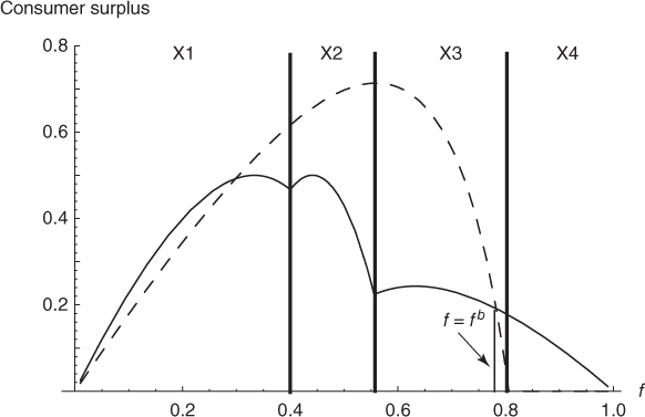
Figure 9.7 Consumer surplus comparison with nonuniformly ordered consumer types; smart pipe (solid) versus dumb pipe (dashed);  ,
,  ,
,  ,
,  ,
,  and
and  .
.
Moving on to social welfare, Figure 9.8 indicates that smart pipes lead to a higher social surplus in X4 and a part of X3.

Figure 9.8 Social surplus comparison with nonuniformly ordered consumer types; smart pipe (solid) versus dumb pipe (dashed);  ,
,  ,
,  ,
,  ,
,  and
and  .
.
This figure also shows that dumb pipes can result in a higher social surplus at relatively moderate values of f, for example, in X2. Evidently, the common wisdom regarding which strategy is better from the point of view of the social planner is not applicable in this context as well—depending on the sizes of different market segments, either strategy might result in a higher social surplus.
Theorems 9.6 and 9.8 extend the counterintuitive findings described in the context of uniform ordering to the case of nonuniform ordering. The intuition is still the same. While using smart pipes, the carrier selectively serves the two consumer types; for example, in X4, it restricts service 2 to type-2 consumers only. However, when discrimination across services is not possible, the carrier has to choose between serving type 1 both services there and serving them none. Serving both adequately requires ceding too large a surplus to type 2. The carrier, therefore, finds it preferable to shut out type-1 consumers in X4 while significantly raising the price on type 2 consumers.
9.4 Conclusion
In this chapter, we have examined the economic impacts of service-based discrimination on the market for telecommunication services. We have analyzed a market with discrete consumer types, who may or may not be uniformly ordered with regards to their preferences for various services. We have closely examined—analytically and numerically—how various surpluses behave depending on the pricing strategy used by the carrier. When a carrier employs the smart-pipe strategy, it announces a separate schedule for each service. When it does not discriminate across services, that is, uses the dumb-pipe strategy, it offers just one schedule to price all traffic consumption.
Service-based discrimination is commonly expected to lower consumer and social welfare. It is also expected to lead to a higher producer surplus. We have established—through rigorous economic arguments—that these expectations are often untrue. Specifically, the impact of discrimination is far more complex than often argued, or even imagined. As unambiguously demonstrated in this work, the nature of consumer heterogeneity and relative sizes of different market segments play a pivotal role in determining which strategy would lead to a higher surplus.
Intriguingly, when consumers differ mainly in their incomes and their ordering is thus uniform across services, the expectation that smart pipes harm consumers is true only in situations that involve a few high type consumers and a large number of low type consumers. In fact, despite their natural appeal to consumers, dumb pipes can be detrimental to consumer welfare—in situations, unable to prevent certain consumers from using a service, the carrier may decide to completely forgo them while raising the price on the rest. A similar phenomenon also occurs when consumers differ mainly in their tastes for different services and their ordering is consequently nonuniform. The main lesson, therefore, is that discrimination allows a producer greater flexibility with regards to how it serves different market segments, which may even help it expand coverage, leading to higher surpluses for consumers. This ability of discriminatory pricing to lead to higher consumer welfare gets more pronounced when consumers’ affinity for diversity in use, captured by the parameter ![]() , becomes lower. This is because, when
, becomes lower. This is because, when ![]() is low, the benefits derived from dumb pipes, which primarily arise from the freedom to allocate traffic between services, are also low.
is low, the benefits derived from dumb pipes, which primarily arise from the freedom to allocate traffic between services, are also low.
Another insight that emerges from this chapter is that the perception that discrimination is always beneficial for the producer holds only in the case of uniform ordering. It does not hold in the case of nonuniform ordering. The reason is that an inverse ordering of consumer preferences can turn dumb pipes into a very effective bundling strategy. Equally noteworthy is the insight that service-based discrimination is not always detrimental to social welfare as often believed. The smart-pipe strategy is, in fact, win–win for the carrier and consumers in many situations. The implication is intriguing. The usual arguments about how smart pipes serve as a mechanism for reallocating surplus from consumers to the carrier have little merit. These usual“zero-sum” arguments fail to recognize that smart pipes can indeed drive the social surplus higher, creating the possibility of a higher surplus for everyone.
In summary, the salient contribution of this chapter is that it explains why banning smart pipes may not benefit consumers as expected. Further, it explains why dumb pipes do not always lead to a lower producer surplus or a higher social surplus. All these findings have critical implications for everyone, including carriers, consumers, and policymakers. Consumers need to understand that service-based discrimination can work in their favor before they extend unqualified support for a ban on discrimination, or they embrace open platforms with the hope of rendering such discrimination ineffective. Likewise, policymakers should consider the negative impacts a ban on discrimination may produce, including the most unexpected impact of a lower surplus for everyone. A carrier should also note that smart pipes are not necessarily more profitable—they can indeed be suboptimal when consumers are nonuniformly ordered.
This chapter also contributes towards the broader debate on net neutrality. In particular, it sheds light on the issue of neutrality with respect to different services that use the same communication network. Contrary to what supporters of neutrality may claim, the results above all point to the fact that when assessing economic impacts of neutrality, relying on the prevalent wisdom can be futile. Analytical models that rest on well-tested economic theories are desired for proper evaluation of likely consequences.
A word on extending this work to competitive settings is in order now. One way to model a firm, which is not a monopoly but has substantial pricing power, could be to use slightly different participation (Individual Rationality) constraints. So far we have assumed that a consumer must get a nonnegative utility from any plan he/she purchases. Equivalently, we have implicitly assumed the so-called “outside” utility to be zero. It is possible to imagine a setting where the outside utility is positive, as will be the case if consumers have the ability to switch to alternatives offered by the competing firms. Each consumer will then seek a plan that provides them with a utility at least as large as that obtained from the best of all such alternatives. However, extending the work this way is not at all trival, because many more mathematical possibilities will emerge. For example, if the outside utility for one service is high and that for another is low, under dumb pipes, a consumer may allocate all of his/her purchased traffic to the service with the lower outside utility. Thus, the pricing problem may not have interior solutions, implying that analyses of corner solutions may also become necessary. Interested readers may refer to Reference 20 for additional useful guidelines.
References
- 1. A. Lahiri, R. M. Dewan, and M. Freimer. “The disruptive effect of open platforms on the market for wireless services,” Journal of Management Information Systems, 29(3), 2011, 81–109.
- 2. A. Lahiri, R. M. Dewan, and M. Freimer. “Pricing of wireless services: service pricing vs. traffic pricing,” Information Systems Research, 24(2), 2013, 418–435.
- 3. A. Odlyzko. “The evolution of price discrimination in transportation and its implications for the internet,” Review of Network Economics, 3(3), 2004, 323–346.
- 4. ABC News. Cell phone execs grilled by Senate over texting charges, June 18, 2009. Available at: http://abcnews.go.com/video/playerindex?id=7856703.
- 5. S. Keshav. Testimony of Professor Srinivasan Keshav at the hearing on June 16 at the United States Senate Judiciary Committee, 2009. Available at: http://www.judiciary.senate.gov/hearings/testimony.cfm?id=e655f9e2809e5476862f735da14b66b2/&wit_id=e655f9e2809e5476862f735da14b66b2-0-3.
- 6. W. S. Mossberg. Free my phone. The Wall Street Journal, Oct. 22, 2007. Available at: http://online.wsj.com/article/SB119264941158362317.html.
- 7. R. Jackson. AT&T Android phones from Dell, HTC and Motorola coming soon! Jan. 6, 2010, Available at: http://phandroid.com/2010/01/06/att-android-phones-from-dell-htc-and-motorola-coming-soon/.
- 8. K. Brown and P. J. Alexander. “Bundling in cable television: a pedagogical note with a policy option,” International Journal on Media Management, 6(3), 2004, 162–167.
- 9. W. J. Adam and J. L. Yellen. “Commodity bundling and the burden of monopoly,” Quarterly Journal of Economics, 90(3), 1976, 475–498.
- 10. Y. Masuda and S. Whang. “On the optimality of fixed-up-to tariff for telecommunication service,” Information Systems Research, 17(3), 2006, 247–253.
- 11. I. Friend and M. E. Blume. “The demand for risky assets,” American Economic Review, 65(5), 1975, 900–922.
- 12. P. S. Armington. “A theory of demand for products distinguished by place of production,” IMF Staff Papers, 16(1), 1969, 159–178.
- 13. M. Armstrong. “Price discrimination by a many-product firm,” Review of Economic Studies, 66(1), 1999, 151–168.
- 14. M. Mussa and S. Rosen. “Monopoly and product quality,” Journal of Economic Theory, 18(2), 1978, 301–317.
- 15. M. Katz. “Nonuniform pricing, output and welfare under monopoly,” Review of Economic Studies, 50(1), 1983, 37–56.
- 16. K. W. S. Roberts. “Welfare considerations of nonlinear prices,” Economic Journal, 89(353), 1979, 66–83.
- 17. A. Spence. “Nonlinear prices and welfare,” Journal of Public Economics, 8(1), 1977, 1–18.
- 18. R. Schmalensee. “Output and welfare implications of monopolistic third-degree price discrimination,” American Economic Review, 71(1), 1981, 242–247.
- 19. H. Varian. “Price discrimination and social welfare,” American Economic Review, 75(4), 1985, 870–875.
- 20. M. Armstrong and J. Vickers. “Competitive price discrimination,” RAND Journal of Economics, 32(4), 2001, 1–27.