
Chapter 7
Quantifying the Costs of Customers for Usage-Based Pricing
LÁSZLÓ GYARMATI, RADE STANOJEVIC, MICHAEL SIRIVIANOS, and NIKOLAOS LAOUTARIS
7.1 Introduction
The intense competition among telecom operators is a significant driving force behind the growing popularity of usage-based pricing in communication networks. The competition among the operators results in shrinking profit margins: the operators drop prices in order to attract or retain customers and face continuously increasing traffic volumes. In terms of reduction of capital expense (CAPEX) and operational expense (OPEX), the advancements in the technology are not able to keep up with the speed of the increase in traffic. As a consequence, prices offered to customers should take into account any induced expenses to sustain the profitability of the network operators.
Although operators have incentives to move toward usage-based pricing schemes, customers are also paying more attention to their expenses given the recent state of the global economy: they do not want to subsidize the costs of others. To meet the expectations toward usage-based pricing, operators have to understand the cost of their infrastructure and be aware as to how individual customers affect these costs. Understanding and optimizing the total cost of ownership (TCO) of a network, that is, both CAPEX and OPEX, is an important aspect of network operations, and therefore, it has received substantial attention from procurement, network development, and network planning departments of large telcos [1]. However, the impact of individual customers on the cost of the network is much less understood because of reasons such as difficulties of monitoring and nonlinearities of cost–capacity functions.
It is crucial to quantify how individual customers affect the TCO of a network as this can be used to design better tariff schemes that reflect the usage and costs of the customers. For example, a customer could receive discounts if it inflicts low costs or charged more in the opposite case. In this chapter, we focus on the quantification of the customers’ costs in communication networks, that is, how an operator should share the cost of the infrastructure among its customers. The structure of the chapter is as follows. First, we review the cost of the network infrastructure and also how this cost is affected bythe aggregate traffic of the customers (Section 7.2). Afterwards, we introduce a metric, namely, discrepancy, that quantifies the differences of cost-sharing policies (Section 7.3). The forthcoming sections introduce several factors that impact the quantification of the customers’ costs. In all the cases, we apply the introduced methodologies on real-world datasets: we derive the costs of the customers of a large backbone network. Section 7.8 discusses related work while the conclusion is arrived at in Section 7.9.
7.2 The Cost of a Customer in a Network
We start with an example to show the pitfalls of the quantification of customers’ cost in a communication network. In Figure 7.1, we depict a toy infrastructure used by two customers. The customers access web services using their mobile devices. Let us assume that the aggregate cost of the infrastructure is $21k; we compute this by summing up all the expenditure of the parts of the network. Now we have to share this amount between the customers. A straightforward way is to look at the volume of the traffic they inject into the network and share the cost of the infrastructure proportional to this. As both customers have traffic of 10 Mbps, they both have a cost of $10.5k. This is a simple cost-sharing policy; however, it has some limitations in terms of fairness. One may ask why should customer 1 partially cover the costs of the other customer? An alternate cost-sharing policy is when we consider exactly which parts of the network were used by which customer. In this way, customer 1 has only $4.5k cost because it uses a link partially with the other customer and an additional one exclusively.

Figure 7.1 Quantifying the costs of the customers is challenging. The customers use different parts of the infrastructure and, hence, can be accounted for diverse costs even of their traffic is identical.
Additional factors impact the quantified cost of the customers including the precise cost of the infrastructure itself. The cost of a network consists of CAPEX and OPEX for all devices present in the network. The CAPEX is the one-time cost paid whenever equipment is bought and installed [1]. It depends on the amount of traffic the device must carry at a specific level of quality of service (QoS). A key observation is that the capacity needed to guarantee a certain QoS depends on the peak traffic that needs to be carried. This is because for a given capacity, QoS is minimized when the traffic peaks. The OPEX corresponds to operational costs such as real estate, energy, and personnel. It also depends on the amount of traffic and the QoS; however, that dependence is more elastic. The cost-sharing policies we discuss are generic enough to capture both CAPEX and OPEX with appropriate parameterization.
Next, we describe how we determine the aggregate cost that the sharing policies distribute. A network consists of various network devices, for example, routers and links. Let ![]() denote the set of devices of the network. Let
denote the set of devices of the network. Let ![]() denote the traffic volume of customer
denote the traffic volume of customer ![]() on network device
on network device ![]() during the time interval
during the time interval ![]() . Furthermore, let
. Furthermore, let ![]() denote the cost of network device
denote the cost of network device ![]() . The cost of a specific device depends on the maximum amount of traffic that it has to carry during a certain time interval. Thus, we obtain
. The cost of a specific device depends on the maximum amount of traffic that it has to carry during a certain time interval. Thus, we obtain ![]() by examining the available capacity rates of the device (e.g., 1 and 10 Gbps) and then using the cost of the smallest device whose capacity satisfies the requested service-level agreement (SLA) for the given traffic demand. For example, the operator fulfills its SLA by upgrading its devices when utilization hits the 50% threshold. To this end, we assume that the costs follow a step function
by examining the available capacity rates of the device (e.g., 1 and 10 Gbps) and then using the cost of the smallest device whose capacity satisfies the requested service-level agreement (SLA) for the given traffic demand. For example, the operator fulfills its SLA by upgrading its devices when utilization hits the 50% threshold. To this end, we assume that the costs follow a step function ![]() . Thus, the cost of device
. Thus, the cost of device ![]() is
is

7.2.1 Datasets used in the Case Studies
In the remainder of the chapter, we introduce several factors that influence the quantified cost of the customers. We also present case studies to illustrate the applicability of the methodology in real-world scenarios. To this end, we use several datasets from a tier-1 backbone network, which interconnects with other Internet Service Providers (ISPs) that it serves. In our dataset, the network consists of tens of points of presence (PoPs) and eachcustomer connects to the network at one or more PoPs through one or more interfaces. Overall, the datasets contain the per-link and per-customer traffic statistics of more than 1000 links over a period of 3 weeks, with a 2-h granularity (i.e., reporting volumes sent and received within 2 h). For additional details on the datasets, we refer to Reference 2.
The cost of a network link depends, on the one hand, on the capacity of the interface, that is, how much traffic it is capable of forwarding. On the other hand, the geographic location and the applied technology have an impact as well. Hardware costs, energy prices, deployment costs, and taxation, among others, contribute to the cost of a network device. Thereby, it is challenging to accurately quantify the cost of every single device. To estimate the cost of the network links, we use a wholesale point-to-point transport price database. In our empirical analysis, we apply the prices of network links with different bandwidth, ranging from E-1 (2 Mbps) throughout STM-4 (622 Mbps) and 2.5G waves to 40G waves (40,000 Mbps). The costs of these links define a step function for the network expenditures.
Although we analyze a backbone network as a case study, we emphasize that the methodology we use to quantify the costs of the customers is general enough to be applied in access networks [3] or for the whole end-to-end traffic of the customers.
7.3 Discrepancy, The Metric of Comparing Different Cost-Sharing Policies
The operator can quantify the cost of the customers in numerous ways using cost-sharing policies. We will present several orthogonal factors that could be combined arbitrarily to create cost-sharing policies that are in line with the objectives of the operator. The quantification of the customers’ costs is a multifacet problem covering the following questions:
- How do we compute the costs of the customers?
- Where do we meter the traffic?
- What is the impact of the diverse costs of the devices?
- Who is liable for the incurred costs?
Before addressing these questions and introducing the appropriate types of discrepancies, we first introduce the metric we use to quantify the discrepancies of a pair of cost-sharing procedures. Let ![]() denote the set ofcustomers who utilize resources in the network. Let
denote the set ofcustomers who utilize resources in the network. Let ![]() and
and ![]() denote the sets of costs allocated to each customer using two different cost-sharing policies. It holds that
denote the sets of costs allocated to each customer using two different cost-sharing policies. It holds that ![]() . Accordingly,
. Accordingly, ![]() denotes the cost of customer
denotes the cost of customer ![]() quantified based on the first cost-sharing policy while
quantified based on the first cost-sharing policy while ![]() represents customer
represents customer ![]() 's cost based on the second policy. We define the discrepancy of the costs of customer
's cost based on the second policy. We define the discrepancy of the costs of customer ![]() as
as
We use this measure of discrepancy because it describes the relation of the costs with a simple, comprehensible value. In the case studies, we use several statistics of the customers’ individual discrepancies to quantify the discrepancy of two cost-sharing policies including the 95th percentile and the median.
Illustrative Example
Let us assume that three customers utilize the resources of the network with costs presented in Table 7.1. The operator quantified the costs of the customers using two cost-sharing policies. As we compute the discrepancy of the policies for each customer, we gain both individual and aggregate insights. For example, the two policies are identical in case of the third customer; however, the discrepancy of the policies is 4 in case of the second customer, that is, the cost of the customer is four times higher in case of policy A. For aggregate insights, we investigate the distribution of the discrepancies, for example, the median discrepancy of the policies is 2.
Table 7.1 Illustrative Example for Computing Discrepancies
| Cost Based on | Cost Based on | ||
| Policy A | Policy B | Discrepancy | |
| Customer 1 | 150 | 300 | 2 |
| Customer 2 | 200 | 50 | 4 |
| Customer 3 | 150 | 150 | 1 |
We quantify the costs of the customers using two cost-sharing policies and derive the discrepancies of these policies.
7.4 How Do We Compute the Costs of the Customers?
The first source of discrepancies in some cost allocation methods is the function that the operator uses to compute the contribution of the customers to the aggregate cost (i.e., F-discrepancy). We next present four policies that strike different balances between precision and resource needs. We consider these methods because operators apply some of these policies (e.g., the 95Percentile-Customer and the Aggregate-Peak-Device) in practice to determine the costs a customer inflicts and consequently the price the customers pays. For example, one can easily map some of the tariffs (e.g., based on the purchased raw capacity or on the 95th percentile of the traffic) used in practice to the introduced policies (e.g., Volume-Customer and 95Percentile-Customer).
- Volume-Customer. We measure the amount of data that a single customer sends on a specific network device (e.g., on a single link) for the whole analyzed time period. Afterwards, we share the cost of the device proportionally to the traffic volumes of the customers using it. Hence, the cost of customer
 for device
  is
7.3
is
7.3
- 95Percentile-Customer. We distribute the cost of the device proportional to the 95th percentile [4] of the customers’ traffic that traverses the particular device:
7.4where

 denotes the 95th percentile of the arguments.
 - Peak-Customer. Under this policy, we share the expenditure of the network device proportional to the customers’ maximum usage volumes for the given time interval:
7.5

- Aggregate-Peak-Device. Operators plan the capacity of the network based on the maximum utilization, for example, the 50% of the capacity of a device is larger than the expected maximum of the traffic that traverses it. Accordingly, we distribute the cost of the devices based on the contribution of individual customers to the peak utilization. Assuming that the peak utilization of device
 happens at time step
  , we allocate the following cost to customer
  as
7.6
as
7.6
We evaluate F-discrepancies by comparing a policy with Aggregate-Peak-Device, which shares the costs in a fair way when it is guaranteed that new unallocated capacity from an upgrade will soon find a customer to amortize it. The F-discrepancies of the policies arise from the misalignment of traffic peaks: the peak of a customer's traffic may not coincide with the peak of the aggregate traffic the device carries. Before presenting a date-driven evaluation of F-discrepancies, we first illustrate the introduced policies.
Illustrative Example
Let us assume that two customers utilize device ![]() with traffic volumes depicted in Figure 7.2. On the basis of the time series of the customers, we compute their costs, that is, what portion of the total cost of the device is related to each customer. The percentages of the cost that customer 1 covers are 69.9%, 56.2%, 60%, and 53.3% of the total cost of the device for the Volume-Customer, Peak-Customer, 95Percentile-Customer, and Aggregate-Peak-Device policies, respectively. In terms of discrepancies these are 1.31, 1.05, 1.13, and 1.0 having Aggregate-Peak-Device as reference. We use the introduced formulae of the policies to compute the shares of the customers. For example, in case of the 95Percentile-Customer policy, customer 1 has a traffic of
with traffic volumes depicted in Figure 7.2. On the basis of the time series of the customers, we compute their costs, that is, what portion of the total cost of the device is related to each customer. The percentages of the cost that customer 1 covers are 69.9%, 56.2%, 60%, and 53.3% of the total cost of the device for the Volume-Customer, Peak-Customer, 95Percentile-Customer, and Aggregate-Peak-Device policies, respectively. In terms of discrepancies these are 1.31, 1.05, 1.13, and 1.0 having Aggregate-Peak-Device as reference. We use the introduced formulae of the policies to compute the shares of the customers. For example, in case of the 95Percentile-Customer policy, customer 1 has a traffic of ![]() Mbps while the cumulative traffic is
Mbps while the cumulative traffic is ![]() Mbps resulting in 60% cost share. The main cause behind the discrepancies of the costs are the misalignment of the customers’ peak, and that the different policies consider diverse parts of the time series to compute a value that describes the traffic of the customer.
Mbps resulting in 60% cost share. The main cause behind the discrepancies of the costs are the misalignment of the customers’ peak, and that the different policies consider diverse parts of the time series to compute a value that describes the traffic of the customer.

Figure 7.2 Illustrative example for F-discrepancies. The misalignment of the customers’ peak causes cost differences across policies. (a) Toplogy and (b) traffic pattern of  .
.
The introduced policies quantify the cost of the customers using different functions on a per-device basis. The F-discrepancies of the customers emerge at two different levels.
- Device-Level Discrepancies. The discrepancy among different policies based on the customers’ costs is computed separately for each network device. In this case, the set of costs is
7.7and has cardinality

 . For example, the F-discrepancy of customer
  in case of policies
  and
and  is
is  .
. - Network-Level Discrepancies. We first summarize the costs of a customer over all the devices of the network, that is, we compute the total cost of each customer. Afterwards, we compute the discrepancies of the policies. In this case, the set of the costs over which we compute the discrepancies is
7.8and has cardinality

 . For example, for policies
  and
and  , the F-discrepancy of customer
  is
is  .
.
7.4.1 Case Study: F-Discrepancy in Backbone Networks
In the case studies, we use the datasets introduced in Section 7.2.1 to evaluate the various discrepancies of the cost-sharing policies. We use a uniform cost function for the network devices in this section to focus on the specific properties of the cost-sharing policies.
7.4.1.1 Device-Level F-Discrepancies
To showcase the intricacies of F-discrepancies, we start with an example based on a backbone link between two major PoPs in Europe. The monthly cost of this link is $2163. In Figure 7.3, we plot the amount of this cost attributed to each one of the 10 largest customers according to the four policies. The F-discrepancy, that is, the ratio of the cost computed by the Aggregate-Peak-Device policy and the cost computed by the simpler policy X![]() [Volume-Customer, 95Percentile-Customer, Peak-Customer] is as high as 2.36 for customer 4 in this example. This particular customer impacts the aggregate peak of the device disproportionally more than the other customers when we focus on the traffic volumes of the customers. For several other customers the F-discrepancies are much milder, that is, the different cost-sharing policies are more or less in agreement. In the case of customer 4, the Volume-Customer policy fails by 50% to approximate well the Aggregate-Peak-Device policy (thus, in this particular case, the F-discrepancy is 2). This means that the traffic of this customer is peaky instead of uniformly spread throughout the day.
[Volume-Customer, 95Percentile-Customer, Peak-Customer] is as high as 2.36 for customer 4 in this example. This particular customer impacts the aggregate peak of the device disproportionally more than the other customers when we focus on the traffic volumes of the customers. For several other customers the F-discrepancies are much milder, that is, the different cost-sharing policies are more or less in agreement. In the case of customer 4, the Volume-Customer policy fails by 50% to approximate well the Aggregate-Peak-Device policy (thus, in this particular case, the F-discrepancy is 2). This means that the traffic of this customer is peaky instead of uniformly spread throughout the day.
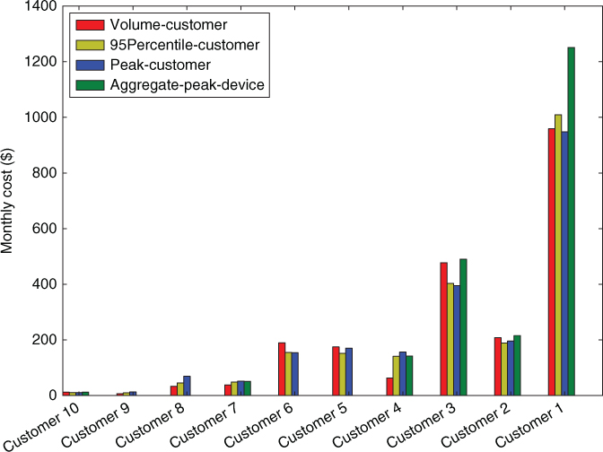
Figure 7.3 Device-level cost of customers for varying cost-sharing policies. Link between two European PoPs.
We now look at F-discrepancies across all customers and all links in our dataset. In Figure 7.4, we plot the F-discrepancies for the three simpler policies and we summarize the main statistics in Table 7.2. The results show generally high F-discrepancies. For example, 60% of the customers are assigned 25% higher or lower cost than the real one they inflict according to Aggregate-Peak-Device. F-discrepancies are particularly high for Volume-Customer and smaller for Peak-Customer and 95Percentile-Customer. The last two policies are sensitive to peaks, albeit those of particular customers instead of peaks of the aggregate traffic on the device. Volume-Customer is even less accurate because it is not looking at any peaks but only at aggregate volume over a longer time scale.

Figure 7.4 Distribution of the device-level F-discrepancies between the simpler cost-sharing policies and the Aggregate-Peak-Device policy. Distributions are based on the percentage of the customers and the traffic (insets). All the policies have high F-discrepancies, especially the F-discrepancies of the Volume-Customer policy are large. (a) Volume-Customer, (b) Peak-Customer, and (c) 95Percentile-Customer.
Table 7.2 Device-Level F-Discrepancies Compared to the Aggregate-Peak-Device Policy
| Method | Median | 95th Percentile | |
| Volume-Customer | 0.592 | 1.372 | 63.07 |
| Peak-Customer | 0.520 | 1.263 | 89.55 |
| 95Percentile-Customer | 0.508 | 1.259 | 80.79 |
To illustrate the differences between the policies, Figure 7.5 depicts a portion of the time series of a link where a large F-discrepancy (![]() ) exists between the Volume-Customer and the Aggregate-Peak-Device policies. The figure shows the traffic pattern of the customer with the large F-discrepancy and the aggregate traffic pattern of the other customers. The traffic of the customer is marginal compared to the traffic of the others, yielding a very low Volume-Customer cost. However, during the peak, the customer with the large discrepancy contributes a significant portion to the aggregate traffic, thereby inducing a
) exists between the Volume-Customer and the Aggregate-Peak-Device policies. The figure shows the traffic pattern of the customer with the large F-discrepancy and the aggregate traffic pattern of the other customers. The traffic of the customer is marginal compared to the traffic of the others, yielding a very low Volume-Customer cost. However, during the peak, the customer with the large discrepancy contributes a significant portion to the aggregate traffic, thereby inducing a ![]() times higher Aggregate-Peak-Device than Volume-Customer cost.
times higher Aggregate-Peak-Device than Volume-Customer cost.

Figure 7.5 Time series of the traffic of a customer with a large ( ) F-discrepancy on a single link. Volume-Customer versus Aggregate-Peak-Device policy.
Summary and Implications
In the case of device-level discrepancies, numerous and substantial F-discrepancies exist. This implies that operators should apply the Aggregate-Peak-Device policy for computing the costs in case of a single device instead of the simpler policies.
7.4.1.2 Network-Level F-Discrepancies
We now examine F-discrepancies in the context of the entire backbone network. We do this by summing the costs of a customer over all the network's devices. We present the relative aggregate costs of the 10 largest customers in Figure 7.6; we consider the largest cost as the baseline. We present the F-discrepancies of the policies in Table 7.3. The results reveal that F-discrepancies at the network level are much smaller than that at the device level. For example, the network-level median F-discrepancies are approximately 40% less than the device-level ones. This is because in large networks, positive and negative cost differences at each device cancel each other out; thus, the cost predictions of the simpler policies become more aligned.
Summary and Implications
F-discrepancies although important for individual links or small networks tend to become less significant for larger networks.

Figure 7.6 Aggregate relative costs of the 10 largest customers; comparison normalized by the largest cost.
Table 7.3 Network-Level F-Discrepancies Compared to the Aggregate-Peak-Device Policy
| Method | Median | 95th Percentile | |
| Volume-Customer | 0.5 | 1.251 | 3.141 |
| Peak-Customer | 0.35 | 1.151 | 12.71 |
| 95Percentile-Customer | 0.37 | 1.181 | 5.046 |
7.5 Where Do We Meter the Traffic?
The traffic metering method is the second source of the discrepancies (i.e., M-discrepancy). The resource requirements of the traffic monitoring tools depend on the resolution of metering. The main cause behind the M-discrepancies is the trade-off that operators face: increasing the precision of the metering improves the validity of the quantified cost; however, this comes with an elevated cost for traffic monitoring. We consider the two corner cases of traffic metering:
- Customer-Ingress (CI). Each customer can have several ingress devices through which it injects its traffic to the network. The operator keeps track of the customers’ usage solely on the ingress devices. This is the least expensive metering method. The operator uses the ingress traffic time series to share the network-wide expenditures among the customers.
- Customer-per-Device (CD). If the operator deploys more advanced network monitoring tools, it can capture the time series of the customers not only on the ingress devices but also on all the devices located in the network. This is the most expensive metering method and is typically done using NetFlow technology, which comes at a high procurement and administration cost. Metering the actual traffic on each network device allows the operator to compute the costs of the customers based on the device-specific time series. Therefore, the operator faces a trade-off: more accurate expenditure sharing versus more cost efficient operation.
We define M-discrepancy as follows. First, we compute the cost of customer ![]() on each device
on each device ![]() using a given cost allocation function (e.g., based on the Volume-Customer policy of Section 7.4), and we compute the network-level cost of customer
using a given cost allocation function (e.g., based on the Volume-Customer policy of Section 7.4), and we compute the network-level cost of customer ![]() as
as ![]() . Second, we compute using the given cost allocation function the customer's share (
. Second, we compute using the given cost allocation function the customer's share (![]() ) of the network's total cost (
) of the network's total cost (![]() ) using the ingress traffic time series of the customers. The total ingress traffic of customer
) using the ingress traffic time series of the customers. The total ingress traffic of customer ![]() is
is ![]() , where
, where ![]() denotes the set of ingress devices that customer
denotes the set of ingress devices that customer ![]() uses. Accordingly, the M-discrepancy of customer
uses. Accordingly, the M-discrepancy of customer ![]() is
is

where ![]() is our metric of discrepancy (Eq. 7.2 ).
is our metric of discrepancy (Eq. 7.2 ).
Illustrative Example
Let us now assume that the customers traffic on ![]() is as we show in Figure 7.7. The network consists of two additional devices:
is as we show in Figure 7.7. The network consists of two additional devices: ![]() on which the traffic of the customers is as depicted in Figure 7.2 and
on which the traffic of the customers is as depicted in Figure 7.2 and ![]() which is solely utilized by customer 1 with a constant traffic of 10 Mbps. For illustration purposes, we separate the two flows of customer 1, one on
which is solely utilized by customer 1 with a constant traffic of 10 Mbps. For illustration purposes, we separate the two flows of customer 1, one on ![]() and the other on
and the other on ![]() , with a dashed line in the Figure 7.7. Let us assume that the traffic on device
, with a dashed line in the Figure 7.7. Let us assume that the traffic on device ![]() can be transmitted on a device with modest capacity while the capacity of
can be transmitted on a device with modest capacity while the capacity of ![]() should be larger. The diverse device capacities imply diverse costs as well. In the case of ingress metering, that is, sharing the cost of the network just based on the traffic of
should be larger. The diverse device capacities imply diverse costs as well. In the case of ingress metering, that is, sharing the cost of the network just based on the traffic of ![]() , the cost of customer 1 is 83.9%, 73.1%, 76%, and 72% of the cost of the whole network for the Volume-Customer, Peak-Customer, 95Percentile-Customer, and Aggregate-Peak-Device policies, respectively. However, if we measure the traffic of the customers on all the devices then shares of costs of customer 1 are 75.9%, 65%, 68%, and 62.7%. If we compare these cost fractions, we encounter large discrepancies caused by the level of the metering.
, the cost of customer 1 is 83.9%, 73.1%, 76%, and 72% of the cost of the whole network for the Volume-Customer, Peak-Customer, 95Percentile-Customer, and Aggregate-Peak-Device policies, respectively. However, if we measure the traffic of the customers on all the devices then shares of costs of customer 1 are 75.9%, 65%, 68%, and 62.7%. If we compare these cost fractions, we encounter large discrepancies caused by the level of the metering.

Figure 7.7 Illustrative example for M-discrepancies: metering traffic only at the ingress link ( ) causes customer 1 to have a larger share of the cost than if we meter at all devices. (a) Topology and (b) traffic pattern of
  .
.
7.5.1 Case Study: M-Discrepancy in Backbone Networks
Similar to F-discrepancies, we use the datasets introduced in Section 7.2.1 and a uniform cost function to analyze M-discrepancies. We compute the discrepancy in the customer's network-level cost derived by (i) metering its traffic at its ingress links (Customer-Ingress or CI) and (ii) metering its traffic on each device that the customer uses (Customer-per-Device or CD). All of the policies result in high M-discrepancies (ratios as high as 34) as summarized in Table 7.4.
Table 7.4 Network-Level M-discrepancies of the Cost-Sharing Policies
| Method | Median | 95th Percentile | |
| Volume-Customer | 0.695 | 1.543 | 34.53 |
| Peak-Customer | 0.752 | 1.738 | 32.34 |
| 95Percentile-Customer | 0.750 | 1.630 | 19.10 |
| Aggregate-Peak-Device | 0.763 | 1.801 | 28.52 |
Comparison of the Customer-Ingress and the Customer-per-Device costs of the customers.
Table 7.5 Discrepancies with the Aggregate-Peak-Device Policy Using Customer-per-Device (Real Traffic) Metering
| Method | Median | 95th Percentile | |
| Volume-Customer + CI | 0.760 | 1.816 | 32.69 |
| Aggregate-Peak-Device + CI | 0.763 | 1.801 | 28.52 |
| Volume-Customer + CD | 0.500 | 1.251 | 3.141 |
| Aggregate-Peak-Device + CD | 0.0 | 1.0 | 1.0 |
Abbreviations: CI, Customer-Ingree; CD, Customer-per-Device.
Up to this point, we analyzed the impact of different discrepancies separately. Next, we quantify the joint effect of F-discrepancies and M-discrepancies, that is, how large can the difference be between the most and the least accurate combination of function and metering schemes. We do this by comparing the network-level costs of customers under the Volume-Customer + CI, Volume-Customer + CD, and Aggregate-Peak-Device + CI policies with the nominally accurate one, namely, the Aggregate-Peak-Device + CD policy. The results are summarized in Table 7.5. The Volume-Customer policy has the smallest M-discrepancy, that is, the median discrepancy of the Customer-Ingress and the Customer-per-Device costs is 1.5. On the contrary, the Aggregate-Peak-Device policy yields the largest M-discrepancies. The reason behind this is twofold. First, when metering traffic at the ingress links, traffic that results in peaks at individual links does not result in peaks of the aggregate ingress traffic. Second, under Customer-Ingress, the Aggregate-Peak-Device policy takes into account only the time interval with the largest aggregate traffic while the peaks of the internal devices may happen in other time intervals neglected by the Aggregate-Peak-Device + CI policy. We observe that under the Aggregate-Peak-Device + CI combination, the costs diverge by at least 25% for 76% of the customers. In addition, we note that under the Volume-Customer + CI policy and metering, the discrepancy can be as high as 32.
Summary and Implications
The level at which the operator meters the traffic of the customers has a large impact on the quantified costs. Therefore, operators should apply sophisticated metering strategies (e.g., network-wide deployment of NetFlow-capable traffic monitoring devices) in order to accurately quantify the costs of the customers. Moreover, the simple methods are no longer aligned with the real cost of the customers (i.e., with the Aggregate-Peak-Customer policy) if the traffic is metered on the ingress links.
7.6 What is the Impact of the Diverse Costs of the Devices?
The third class of discrepancies is related to the total cost of ownership (TCO) of different devices of the network (i.e., TCO discrepancy). Owing to the heterogeneous nature of the network—caused by the geographic and technological differences of its parts—the same traffic patterns imply diverse expenditures for the operator on different devices. Therefore, additional discrepancies occur when we consider the TCO of the network in more detail. The following levels of TCO impact the costs and the discrepancies of the customers:
- Pieces of Cost. Even if the capacities of two particular equipment are equal, their costs can vary significantly because of the technology differences (newer vs older generation), location (cost of shipping), differences in purchase price, ad so on.
- Location-Dependent Costs. The network operator deals with diverse costs at each geographic location where it has a presence. The causes behind the varying costs include but are not limited to the following factors: energy (e.g., the energy price in Germany can be twice as much as that in the United Kingdom), facility costs (e.g., the rental cost of office space in Hong Kong can be four times higher than that in Germany [5]), taxation, and personnel costs.
Contrary to the former types of discrepancies, in the case of the TCO, only network-level discrepancies exist. Formally, we define the network-level TCO discrepancy of customer ![]() as
as

where the first term considers the diverse costs of the devices contrary to the second. ![]() denotes the cost of customer
denotes the cost of customer ![]() in case of device
in case of device ![]() assuming uniform cost across all the devices (
assuming uniform cost across all the devices (![]() ).
).
7.6.1 Case Study: TCO Discrepancy in Backbone Networks
Now we take into account that our dataset (Section 7.2.1) contains a geographically distributed set of links with diverse costs. We compute the TCO discrepancies by computing the ratio between the customers’ costs given links with uniform and diverse costs. In Figure 7.8, we illustrate the TCO discrepancies under the Aggregate-Peak-Device policy. Each customer is affected by the TCO discrepancies. The difference between the two costs can be as high as 5% of the cost of the entire network.

Figure 7.8 The customers’ total costs for the uniform and true link costs using the Aggregate-Peak-Device cost-sharing policy; the size of the circles is proportional to the aggregate traffic volume of the customers.
We report the quantified TCO discrepancies of four policies in Table 7.6. The results show generally extreme TCO discrepancies; some customers have TCO discrepancies as high as ![]() . In addition, 80% of the customers are assigned 25% higher or lower cost when the diverse costs of the links is considered.
. In addition, 80% of the customers are assigned 25% higher or lower cost when the diverse costs of the links is considered.
Table 7.6 Network-Level TCO Discrepancies, That is, the Costs of the Customers Based on Uniform Versus Diverse Link Costs
| Method | Median | 95th Percentile | |
| Volume-Customer | 0.830 | 4.305 | 961.1 |
| Peak-Customer | 0.802 | 4.187 | 933.1 |
| 95Percentile-Customer | 0.817 | 4.079 | 922.4 |
| Aggregate-Peak-Device | 0.840 | 4.019 | 862.1 |
Summary and Implications
TCO discrepancies have a very large impact on the costs of the customers. Cross-subsidization problems arise if the impact of TCO differences is neglected. Network operators are aware of the fact that different parts of their network have different TCOs. The implication of our results is that this diversity should also be reflected in the quantification of the customers’ costs—and eventually in the tariffs too.
7.7 Who is Liable for the Incurred Costs?
On the basis of the discussion of Section 7.2, one may conclude that splitting the cost among customers is straightforward: for each device of the network, each customer should pay in proportion to his/her contribution to the peak traffic carried by the device. Things, however, are not that simple owed to liability complications. If we were to build from scratch a new network for a fixed set of customers of known demand, then the cost attributed to each customer should be proportional to the sum of its contributions to the peaks of individual devices. Splitting costs based on the contribution to the peak is indeed exact but only for this “offline problem.” However, in reality, networks are not deployed as a single event but grow organically with the addition of new customers and the ramping up of their traffic. Under this more realistic case, peak-based cost sharing is not guaranteed to be fair. Consider, for example, the case in which a network is already operating at the maximum utilization allowed by QoS constraints and a small new customer triggers an expensive upgrade that leads to a new network with plentiful unallocated capacity. In Figure 7.9, we illustrate the case when a new customer arrives to the network and pushes the aggregate traffic of the device above the upgrade threshold. Peak-based cost sharing would attribute only a small fraction of the overall cost to the new customer. Is that fair? The answer depends on what happens with the unallocated capacity. If the network can easily sell it to new or existing customers, then indeed it is fair. If, however, selling this leftover capacity is not guaranteed, then the new customer may have a larger liability for the upgrade costs.

Figure 7.9 The traffic of a new customer may increase the aggregate traffic of a device to such an extent that the capacity of the device should be upgraded. Who should cover the elevated costs of the network in such a case?
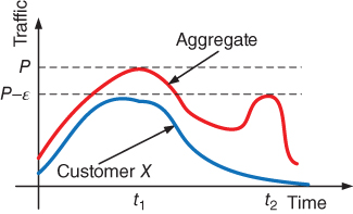
Figure 7.10 The Shapley policy is a robust cost-sharing policy as it takes into account all the local maxima of the aggregate traffic in quantifying the costs of the customers.
The final type of discrepancies is caused by the different types of customer liability (i.e., L-discrepancy). We examine the following policies.
- Aggregate-Peak-Device. This is the already introduced policy that is the measure of fairness when the customer liability is proportional to the aggregate peak of devices.
- Trigger. With this policy, the operator allocates the cost of the device exclusively to the customer that triggered the capacity upgrade. This policy is applied when the operator is not confident that it can sell the newly obtained but unallocated capacity. To this end, the operator utilizes the historical traffic patterns of the customers and their arriving order. For example, the cost of the first customer is equal to the cost of the device that is capable to transmit his traffic demand. We assume that the customers are numbered based on their arriving order while
 denotes the time when the customer started to use the network. Accordingly, the cost of customer
  in case of the Trigger policy is
7.11The main drawbacks of Trigger are (i) it assigns cost only to the customer whose traffic triggers upgrades and 0 to everyone else; therefore, order of arrival can have a huge impact on the costs attributed to a customer; and (ii) it is difficult to compute Trigger because it requires extensive historical data on the order of customer arrival and traffic build up.
in case of the Trigger policy is
7.11The main drawbacks of Trigger are (i) it assigns cost only to the customer whose traffic triggers upgrades and 0 to everyone else; therefore, order of arrival can have a huge impact on the costs attributed to a customer; and (ii) it is difficult to compute Trigger because it requires extensive historical data on the order of customer arrival and traffic build up.
- Shapley. The Shapley cost-sharing policy lies between the two above presented extremes, the Aggregate-Peak-Device and Trigger policies. It assigns to customers partial liability for upgrades, thereby avoiding the all-or-nothing assignments of Triggers. Therefore, it is less strict than Trigger but more strict than Aggregate-Peak-Device because it assigns “averaged” liabilities rather than proportional liabilities based on a single time interval when a device peaks. The main advantage of the Shapley over the Aggregate-Peak-Device policy is that its allocations are more stable than that of the Aggregate-Peak-Device policy in view of customer churn. For example, let us imagine that the aggregate peak traffic of a device is
 and appears at
  (see Fig. 7.10). We also assume that the device at time
  has load
  . Now let us suppose that customer X is responsible for 90% of
  at
at and 1% of
  at
at  . Then if a small
  customer leaves from
  at
at  , then the peak will move to
  and X will go from paying 90% to paying only 1% after a tiny
  perturbation of the aggregate traffic. On the contrary, the Shapley policy is aware of such situations as it takes into account all the local maxima of the aggregate traffic in quantifying the costs of the customers. Under the Shapley policy, the cost of each customer is proportional to its average marginal contribution to the device's total cost. Particularly, let us consider all the possible
  subsets (coalitions) of the customers who utilize resources of the network device
  . The cost of coalition
  depends on the aggregate traffic volume of the participants, that is , it is equal to the cost of a network device that has sufficient capacity:
7.12On the basis of the
depends on the aggregate traffic volume of the participants, that is , it is equal to the cost of a network device that has sufficient capacity:
7.12On the basis of the
 cost function of the coalitions, we compute the Shapley value of customer
  as
7.13where
as
7.13where
 is a permutation of arrival order of the set
  and
and  denotes the set of players who arrived no later than
  . The
. The  Shapley values describe the fair distribution of costs in the case of the
  grand coalition. Fair in a way that it satisfies four intuitive fairness criteria [6–8]. We quantify the cost of customer
  based on its Shapley value for the device
  as
7.14
as
7.14
Illustrative Example
We present the traffic patterns of two customers and the thresholds where the capacity of the device needs to be upgraded in Figure 7.11. Customer 1 is liable for 53.3% and 87.5% of the cost of the device in case of the Aggregate-Peak-Device and Shapley policies, respectively. Thus, the discrepancy is 1.64. The peak of the aggregate traffic happens in a time step where the customers’ traffic volumes are balanced. Although there are local maxima where the traffic of customer 2 is small, it is not considered by the Aggregate-Peak-Device policy. From a Shapley policy viewpoint, the traffic peak of customer 1 is too large to be transmitted with a lower capacity device, that is , its traffic is mainly responsible for the total cost of the device. If we assume that customer 1 arrived first, it causes 100% of the costs according to the Trigger policy because its peak needs a larger-capacity device whose leftover capacity can be used by customer 2 afterwards.

Figure 7.11 Illustrative example for L-discrepancies. The capacity thresholds of device  are shown with dashed lines. (a) Topology and (b) traffic pattern of
  .
.
Customers can have both device- or network-level L-discrepancies, depending on whether we consider the costs of the customers on particular devices (e.g., ![]() ) or on the aggregate (e.g.,
) or on the aggregate (e.g., ![]() ).
).
7.7.1 Case Study: L-Discrepancy in Backbone Networks
Out of the three policies described earlier, one, the Trigger policy, requires historic information on customer arrival events as well as customer traffic information on long time scales that relate to network upgrade events. As we do not have full historic information on all the links, we omit the analysis of the Trigger policy in this case study.
7.7.1.1 Device-Level L-Discrepancies
We present the L-discrepancies in Table 7.7 by computing the ratio between Shapley and the Aggregate-Peak-Device policies. L-discrepancies are quite high (ratios up to 472) pointing to the fact that liability can bias significantly the cost-sharing picture that a telco has. For example, the difference between the costs of the Shapley and the Aggregate-Peak-Device policies is substantial: the median ratio of the costs is 1.5; however, in some cases, the ratio can be larger than 400.
Table 7.7 Device-Level L-Discrepancies Compared to the Aggregate-Peak-Device Policy
| Method | Median | 95th Percentile | |
| Shapley | 0.674 | 1.497 | 472.4 |
We present in Figure 7.12 a part of the time series of a customer with a large L-discrepancy (![]() ) along with the aggregate time series of the other customers who utilize the same link. The dashed horizontal lines denote the traffic volumes where the capacity of the link needs to be upgraded. The traffic of the customer is small enough to be transmitted over a link with lower capacity. However, the traffic of the other customers pushes the link to have larger capacity and thus larger cost. The Shapley policy considers this fact when it computes the average marginal contribution of the customer. As a result, the cost of the customer is less if we compute it based solely on time of the largest utilization of the device. On the contrary, the Aggregate-Peak-Customer policy focuses only on the time interval when the link has its aggregate peak. The particular customer has significant share of the aggregate peak and thus of the cost of the link according to the Aggregate-Peak-Customer. This, however, masks who is responsible for the link's larger capacity.
) along with the aggregate time series of the other customers who utilize the same link. The dashed horizontal lines denote the traffic volumes where the capacity of the link needs to be upgraded. The traffic of the customer is small enough to be transmitted over a link with lower capacity. However, the traffic of the other customers pushes the link to have larger capacity and thus larger cost. The Shapley policy considers this fact when it computes the average marginal contribution of the customer. As a result, the cost of the customer is less if we compute it based solely on time of the largest utilization of the device. On the contrary, the Aggregate-Peak-Customer policy focuses only on the time interval when the link has its aggregate peak. The particular customer has significant share of the aggregate peak and thus of the cost of the link according to the Aggregate-Peak-Customer. This, however, masks who is responsible for the link's larger capacity.

Figure 7.12 Time series of a customer with large ( ) L-discrepancy (Shapley vs Aggregate-Peak-Device policy). The dashed lines represent the traffic volumes where the capacity of the link needs to be upgraded.
7.7.1.2 Network-Level L-Discrepancies
We show the network-level L-discrepancies in Table 7.8. At the network level, the number and the magnitude of the L-discrepancies is smaller than that at the device level. Nevertheless, for more than 50% of the customers, the costs are off by at least 25%. The median L-discrepancies of the policies are notable too.
Table 7.8 Network-Level L-Discrepancies Compared to the Aggregate-Peak-Device Policy
| Method | Median | 95th Percentile | |
| Shapley | 0.54 | 1.316 | 179.3 |
Summary and Implications
The liability of network upgrades plays an important role in the quantification of the costs of customers. The implication of the results is that if the network is not built in one shot but is rather organically grown and upgraded, then the Aggregate-Peak-Customer policy may induce cross-subsidization problems: customers may be accounted for costs of upgrades for which they are not liable (or not in that degree). From a customer point of view, this cross-subsidization may not be tolerated in a long run, given the competitive environment of communication networks. That is, the customers may select other operator where they are not liable for the costs of others. From the operator point of view, the large L-discrepancies dictate that it needs to take them under serious consideration. If it is anticipated that the market for data services will be healthy, the operator should choose the Aggregate-Peak-Device policy. If, however, it expects difficulties in selling its capacity, our results indicate that Shapley should be the policy of choice.
7.8 Related Work
We refer to the textbook of Courcoubetis and Weber [9] for a thorough treatment of pricing in communication networks. More detailed analyses of the challenge of cost sharing in backbone networks were carried out in References 2 and 10.
Several studies investigated how to reduce the transit costs including ISP peering [11–13], CDNs [14], P2P localization [15], and traffic smoothing [16]. Dimitropoulos et al. [4] presented a comprehensive analysis of the 95th percentile pricing. A proposal by Laoutaris et al. [17, 18] showed how traffic can be transferred in the network without increasing the 95th percentile of the customers. A recent proposal by Stanojevic et al. [19] proposes to the customers of transit providers to form a coalition to reduce their transit costs. Valancius et al. [20] show that a small number of pricing tiers are enough to extract close-to-optimal efficiency in the transit provider. Motiwala et al. [21] developed a cost model that operators can use to evaluate the costs of their routing and peering decisions. The net neutrality debate is in many ways related to the question of who is responsible for the costs in the network [22].
Owing to the desirable fairness properties [6–8] of the Shapley value [23], recent studies proposed pricing and cost-sharing mechanisms using Shapley values. Briscoe [24, 25] motivates the usage of mechanisms that share the costs of the users fairly as a way to reduce widely known cross-subsidization (the phenomenon in which a small set of customers is subsidized by a large fraction of other customers of the service) of the common infrastructure that often happens in the communication networks [26]. Stanojevic et al. [27] investigated the cross-subsidization of cellular subscribers from a service plan selection point of view. Cooperative approaches for cost sharing are investigated in case of interdomain routing [28, 29], and IP multicast [6, 7]. Ma et al. [30, 31] presented a fair revenue sharing method for ISPs that quantifies the importance of each ISP in the Internet ecosystem. The work of Stanojevic et al. [3] empirically investigated the temporal usage effects using the Shapley and the 95Percentile-Customer method in case of asymmetric digital subscriber line (ADSL) subscribers.
7.9 Conclusions
Network operators need to know accurately the costs of their customers to apply smart data pricing schemes in practice. Despite the widespread availability of big data infrastructures, the quantification of the costs of individual customers is a challenging task in communication networks. This chapter provided a thorough analysis of four nontrivial underlying mechanism impacting the quantification of the costs. The influencing factors include temporal/spatial characteristics of the customers, nonlinear cost–capacity relationships, measurement infrastructure issues, and high variability of the component costs. On the basis of the findings of our case studies, usage-based tariffs should include device-level expenditures and measurements to assure their accuracy and fairness.
References
- 1. W. B. Norton. The Internet Peering Playbook: Connecting to the Core of the Internet. DrPeering Press, 2012.
- 2. L. Gyarmati, R. Stanojevic, M. Sirivianos, and N. Laoutaris. Sharing the cost of backbone networks: cui bono? In Proceedings of the 2012 ACM Conference on Internet Measurement Conference, IMC ’12, pp. 509–522, New York, NY, USA, 2012. ACM.
- 3. R. Stanojevic, N. Laoutaris, and P. Rodriguez. On economic heavy hitters: shapley value analysis of 95th-percentile pricing. In Proceedings of the 10th ACM SIGCOMM Conference on Internet Measurement, IMC ’10, pp. 75–80, New York, NY, USA, 2010. ACM.
- 4. X. Dimitropoulos, P. Hurley, A. Kind, and M. Stoecklin. “On the 95-percentile billing method,”. In S. Moon, R. Teixeira, and S. Uhlig, eds., Passive and Active Network Measurement, Lecture Notes in Computer Science, vol. 5448, Springer Berlin, Heidelberg, 2009, pp. 207–216.
- 5. Cushman & Wakefield. Office Space Across the World, 2012.
- 6. A. Archer, J. Feigenbaum, A. Krishnamurthy, R. Sami, and S. Shenker. “Approximation and collusion in multicast cost sharing,” Games and Economic Behavior, 47(1), 2004, 36–71.
- 7. J. Feigenbaum, C. H. Papadimitriou, and S. Shenker. “Sharing the cost of multicast transmissions,” Journal of Computer and System Sciences, 63(1), 2001, 21–41.
- 8. H. Moulin and S. Shenker. “Strategyproof sharing of submodular costs: budget balance versus efficiency,” Economic Theory, 18, 2001, 511–533. Doi: 10.1007/PL00004200.
- 9. C. Courcoubetis and R. Weber. Pricing and Communications Networks. John Wiley & Sons, Ltd, 2003, West Sussex, England.
- 10. L. Gyarmati, M. Sirivianos, and N. Laoutaris. Simplicity vs Precision: sharing the cost of backbone networks. In NetEcon 2012 - Seventh Workshop on the Economics of Networks, Systems, and Computation, 2012.
- 11. B. Augustin, B. Krishnamurthy, and W. Willinger. Ixps: mapped? In Proceedings of the 9th ACM SIGCOMM Conference on Internet Measurement Conference, IMC ’09, pp. 336–349, New York, NY, USA, 2009. ACM.
- 12. A. Dhamdhere and C. Dovrolis. The internet is flat: modeling the transition from a transit hierarchy to a peering mesh. In Proceedings of the 6th International Conference, Co-NEXT ’10, pp. 21:1–21:12, New York, NY, USA, 2010. ACM.
- 13. A. Dhamdhere, C. Dovrolis, and P. Francois. A value-based framework for internet peering agreements. In Teletraffic Congress (ITC), 2010 22nd International, 2010.
- 14. L. Qiu, V. N. Padmanabhan, and G. M. Voelker. On the placement of web server replicas. In IEEE INFOCOM, pp. 1587–1596, 2001.
- 15. D. R. Choffnes and F. E. Bustamante. Taming the torrent: a practical approach to reducing cross-ISP traffic in peer-to-peer systems. In Proceedings of the ACM SIGCOMM 2008 Conference on Data Communication, SIGCOMM ’08, pp. 363–374, New York, NY, USA, 2008. ACM.
- 16. M. Marcon, M. Dischinger, K. P. Gummadi, and A. Vahdat. The local and global effects of traffic shaping in the internet. In Third International Conference on Communication Systems and Networks (COMSNETS), 2011.
- 17. N. Laoutaris, G. Smaragdakis, P. Rodriguez, and R. Sundaram. Delay tolerant bulk data transfers on the internet. In Proceedings of the Eleventh International Joint Conference on Measurement and Modeling of Computer Systems, SIGMETRICS ’09, pp. 229–238, New York, NY, USA, 2009. ACM.
- 18. N. Laoutaris, M. Sirivianos, X. Yang, and P. Rodriguez. Inter-data center bulk transfers with netstitcher. In Proceedings of the ACM SIGCOMM 2011 Conference, SIGCOMM ’11, pp. 74–85, New York, NY, USA, 2011. ACM.
- 19. R. Stanojevic, I. Castro, and S. Gorinsky. Cipt: using tuangou to reduce ip transit costs. In Proceedings of the Seventh Conference on Emerging Networking Experiments and Technologies, CoNEXT ’11, pp. 17:1–17:12, New York, NY, USA, 2011. ACM.
- 20. V. Valancius, C. Lumezanu, N. Feamster, R. Johari, and V. V. Vazirani. How many tiers? Pricing in the internet transit market. In Proceedings of the ACM SIGCOMM 2011 Conference, SIGCOMM ’11, pp. 194–205, New York, NY, USA, 2011. ACM.
- 21. M. Motiwala, A. Dhamdhere, N. Feamster, and A. Lakhina. “Towards a cost model for network traffic,” SIGCOMM Computer Communication Review, 42(1), 2012, 54–60.
- 22. K. C. Claffy. “Network neutrality”: the meme, its cost, its future,” SIGCOMM Computer Communication Review, 41(5), 2011, 44–45.
- 23. L. S. Shapley. “A Value for n-Person Games,” In Annals of Mathematical Studies, H. W. Kuhn and A. W. Tucker (eds.), 1953, pp. 307–318.
- 24. B. Briscoe. “Flow rate fairness: dismantling a religion,” SIGCOMM Computer Communication Review, 37(2), 2007, 63–74.
- 25. B. Briscoe. “A fairer, faster internet,” IEEE Spectrum, 45(12), 2008, 42–47.
- 26. K. Cho, K. Fukuda, H. Esaki, and A. Kato. The impact and implications of the growth in residential user-to-user traffic. In SIGCOMM ’06, pp. 207–218, New York, NY, USA, 2006. ACM.
- 27. R. Stanojevic, V. Erramilli, and K. Papagiannaki. Cognitive bias in network services. In Proceedings of the 11th ACM Workshop on Hot Topics in Networks, HotNets-XI, pp. 49–54, New York, NY, USA, 2012. ACM.
- 28. R. Mahajan, D. Wetherall, and T. Anderson. Negotiation-based routing between neighboring ISPs. In Proceedings of the 2nd Conference on Symposium on Networked Systems Design & Implementation - Volume 2, NSDI’05, pp. 29–42, Berkeley, CA, USA, 2005. USENIX Association.
- 29. G. Shrimali, A. Akella, and A. Mutapcic. “Cooperative interdomain traffic engineering using Nash bargaining and decomposition,” IEEE/ACM Transactions on Networking, 18(2), 2010, 341–352.
- 30. R. T. B. Ma, D. M. Chiu, J. C. S. Lui, V. Misra, and D. Rubenstein. Internet economics: the use of shapley value for ISP settlement. In Proceedings of the 2007 ACM CoNEXT Conference, CoNEXT ’07, pp. 6:1–6:12, New York, NY, USA, 2007. ACM.
- 31. R. T. B. Ma, D.-M. Chiu, J. C. S. Lui, V. Misra, and D. Rubenstein. On cooperative settlement between content, transit and eyeball internet service providers. In Proceedings of the 2008 ACM CoNEXT Conference, CoNEXT ’08, pp. 7:1–7:12, New York, NY, USA, 2008. ACM.