CHAPTER 18
Distributed Algorithms
In a paper published in 1965, Gordon E. Moore noticed that the number of transistors on integrated circuits roughly doubled every two years between the invention of the integrated circuit in 1958 and 1965. From that observation, he predicted that the trend would continue for at least another 10 years. This prediction, which is now known as Moore's Law, has proven amazingly accurate for the last 50 years, but the end may be in sight.
The size of the objects that manufacturers can put on a chip is reaching the limits of the current technology. Even if manufacturers find a way to put even more on a chip (they're quite clever, so it's certainly possible), eventually transistors will reach quantum sizes where the physics becomes so weird that current techniques will fail. Quantum computing may be able to take advantage of some of those effects to create amazing new computers, but it seems likely that Moore's Law won't hold forever.
One way to increase computing power without increasing the number of transistors on a chip is to use more than one processor at the same time. Most computers for sale today contain more than one central processing unit (CPU). Often they contain multiple cores—multiple CPUs on a single chip. Clever operating systems may be able to get some use out of extra cores, and a good compiler may be able to recognize parts of a program that can be executed in parallel and run them on multiple cores. To really get the most out of multiple CPU systems, however, you need to understand how to write parallel algorithms.
This chapter explains some of the issues that arise when you try to use multiple processors to solve a single problem. It describes different models of parallel processing and explains some algorithms and techniques you can use to solve parallelizable problems more quickly.
Types of Parallelism
There are several models of parallelism, and each is dependent on its own set of assumptions, such as the number of processors you have available and how they are connected. Currently distributed computing is the most common model for most people, but other forms of parallel computing are interesting, so this chapter spends a little time describing some of them, beginning with systolic arrays. You may be unable to use a large systolic array, but understanding how one works may give you ideas for other algorithms you might want to write for a distributed system.
Systolic Arrays
A systolic array is an array of data processing units (DPUs) called cells. The array could be one-, two-, or even higher-dimensional.
Each cell is connected to the cells that are adjacent to it in the array, and those are the only cells with which it can communicate directly.
Each cell executes the same program in lockstep with the other cells. This form of parallelism is called data parallelism because the processors execute the same program on different pieces of data. (The term “systolic array” comes from the fact that data is pumped through the processors at regular intervals, much as a beating heart pumps blood through the body.)
Systolic arrays can be very efficient, but they also tend to be very specialized and expensive to build. Algorithms for them often assume that the array holds a number of cells that depends on the number of inputs. For example, an algorithm that multiplies N×N matrices might assume it can use an N×N array of cells. That assumption limits the size of the problem you can solve to the size of the array you can build.
Although you may never use a systolic array, their algorithms are fairly interesting, so this section presents one to give you an idea of how they work.
Suppose you want to sort a sequence of N numbers on a one-dimensional systolic array containing N cells. The following steps describe how each cell can process its data:
- To input the first half of the numbers, repeat N times:
- Each cell should move its current value to the right.
- If this is an odd-numbered step, push a new number into the first cell. If this is an even-numbered step, do not add a new number to the first cell.
- To input the second half of the numbers, repeat N times:
- If a cell contains two values, it should compare them, move the smaller value left, and move the larger value right.
- If the first cell contains one number, it should move it right.
- If the last cell contains one number, it should move it left.
- If this is an odd-numbered step, push a new number into the first cell. If this is an even-numbered step, do not add a new number to the first cell.
- To output the sorted list, repeat N times:
- If a cell contains two values, it should compare them, move the smaller value left, and move the larger value right.
- If a cell contains one value, it should move it left.
Figure 18-1 shows this algorithm sorting the values 3, 4, 1, and 2 with an array of four cells. The first row in the figure shows the empty array of cells, with the numbers to be sorted on the left.
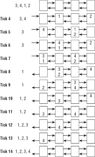
Figure 18-1: A systolic array of four cells can sort four numbers in 14 ticks.
The first four systolic ticks push the first two values (2 and 1) into the array. (The figure calls them “ticks” so that you don't confuse them with the algorithm's steps.) These ticks correspond to Step 1 in the algorithm.
The interesting part of the algorithm begins with tick 5. This is where Step 2 of the algorithm begins. During this tick, the algorithm pushes the new value 4 into the first cell. At this point the third cell contains the values 1 and 2. It compares them, moves the smaller value 1 left, and moves the larger value 2 right.
In tick 6, the second cell compares the values 4 and 1. It moves 1 left and moves 4 right. During this tick the algorithm also moves the last value, 3, into the first cell.
In tick 7, the first cell compares 3 and 1, moves 1 left to the output list, and moves 3 right. At the same time, the third cell compares 4 and 2, moves 2 left, and moves 4 right.
In tick 8, the second cell compares 3 and 2, moves 2 left, and moves 3 right. The last cell moves 4 left.
In tick 9, Step 3 of the algorithm begins. The first cell outputs the value 2. The third cell compares 3 and 4, moves 3 left, and moves 4 right.
In ticks 10 through 14, the cells contain at most one value, so they move their values left, eventually adding them to the sorted output.
This may seem like a lot of steps to sort four items, but the algorithm would save time if the list of numbers were larger. For N items, the algorithm needs N steps to move half of the numbers into the array (Step 1), N more steps to move the rest of the numbers into the array (Step 2), and N more steps to pull out the last of the sorted values.
The total number of steps is O(3 × N) = O(N), which is faster than the O(N log N) steps required by any nonparallel algorithm that uses comparisons to sort N numbers. Because the numbers are spread across up to N / 2 cells, the cells can perform up to (N / 2)2 comparisons at the same time.
This algorithm has a couple of interesting features. First, in tick 7, the last value enters the array, and in tick 8, the first sorted value pops out. Because the first sorted value pops out as soon as the last value is entered, making it seem as if the algorithm is using no time at all to sort the items, this algorithm is called a “zero-time sort.”
Another interesting feature of this algorithm is that only half of its cells contain data at any one time. If you wanted to, you could pack values for a second sequence of numbers into the unused cells and make the array sort two lists at the same time.
Distributed Computing
In distributed computing, multiple computers work together over a network to get a job done. The computers don't share memory, although they may share disks.
Because networks are relatively slow compared to the communication that is possible between CPUs within a single computer, distributed algorithms must try to minimize communication between the computers. Typically a distributed algorithm sends data to the computers, the computers spend some time working on the problem, and then they send back a solution.
Two kinds of distributed environments are cluster and grid computing. A cluster is a collection of closely related computers. Often they are connected by an intranet or a special-purpose network that has limited access to outside networks. For many practical purposes, you can think of a cluster as a giant computer that has unusual internal communications.
In grid computing, the collection of computers is much less tightly integrated. They may communicate over a public network and may even include different kinds of computers running different operating systems.
Communications among the computers in grid computing can be quite slow and may be unreliable. Because the computers are only loosely associated, any given computer may not finish its assigned calculations before its owner shuts it down, so the system needs to be able to reassign subproblems to other computers if necessary.
Despite the drawbacks of relatively slow communications and the unreliability of individual computers, grid computing allows a project to create a “virtual supercomputer” that can potentially apply enormous amounts of processing power to a problem. The following list summarizes some public grid projects:
- MilkyWay@home
http://milkyway.cs.rpi.edu/milkyway
This project is building a very accurate model of the Milky Way galaxy for use in astroinformatics and computer science research. This project's 38,000 or so computers provide about 1.6 petaflops.
- Berkeley Open Infrastructure for Network Computing (BOINC)
This open source project is used by many separate projects to study problems in astrophysics, mathematics, medicine, chemistry, biology, and other fields. Its roughly 600,000 computers provide about 9.2 petaflops.
- Folding@home
This project models protein folding in an attempt to understand diseases such as Alzheimer's, mad cow (BSE), AIDS, Huntington's, Parkinson's, and many cancers. This project's almost 200,000 computers provide about 12 petaflops.
FLOPS
Often the speed of computers that are used to perform intensive mathematical calculations is measured in floating-point operations per second (flops). One teraflop (tflop) is 1012 flops, or 1 trillion flops. One petaflop (pflop) is 1015 flops, or 1,000 teraflops. For comparison, a typical desktop system might be able to run in the 0.25 to 10 gigaflops range.
If you're interested in these projects, visit their web pages to download software that will let your computer contribute CPU cycles when it's idle.
Because the processes on distributed computers can execute different tasks, this approach demonstrates task parallelism. Contrast this with data parallelism, in which the focus is distributing data across multiple processors.
Multi-CPU Processing
Most modern computers include multiple processors. Sometimes these are on separate chips, but often they are multiple cores on a single chip.
CPUs on the same computer can communicate much more quickly than computers in a distributed network, so some of the communications problems that can trouble distributed networks don't apply. For example, a distributed network must pass the least possible data between computers so that the system's performance isn't limited by communication speeds. In contrast, CPUs in the same computer can communicate very quickly, so they can exchange more data without paying a big performance penalty.
Multiple CPUs on the same computer can also access the same disk drive and memory.
The ability to exchange more data and to access the same memory and disks can be helpful, but it also can lead to problems such as race conditions and deadlock. These can happen with any distributed system, but they're most common in multi-CPU systems because it's so easy for the CPUs to contend for the same resources.
Race Conditions
In a race condition, two processes try to write to a resource at almost the same time. The process that writes to the resource second wins.
To see how this can happen, suppose two processes use heuristics to find solutions to the Hamiltonian path problem (discussed in Chapter 17) and then use the following pseudocode to update shared variables that hold the best route found so far and that route's total length:
// Perform heuristics. ... // Save the best solution. If (test_length < BestLength) Then // Save the new solution. ... // Save the new total length. BestLength = test_length End If
The pseudocode starts by using heuristics to find a good solution. It then compares the best total route length it found to the value stored in the shared variable BestLength. If the new solution is better than the previous best, the pseudocode saves the new solution and the new route's length.
Unfortunately, you cannot tell when the multiple processes will actually access the shared memory. Suppose two processes happen to execute their code in the order shown in the following pseudocode timeline:
// Perform heuristics. ... // Perform heuristics. ... // Save the best solution. If (test_length < BestLength) Then // Save the best solution. If (test_length < BestLength) Then // Save the new solution. ... // Save the new solution. ... // Save the new total length. BestLength = test_length End If // Save the new total length. BestLength = test_length End If
The timeline shows the actions performed by process A on the left and those performed by process B on the right.
Process A performs its heuristics, and then process B performs its heuristics.
Process A then executes the If test to see whether it found an improved solution. Suppose for this example that the initial best solution had a route length of 100, and process A found a route with a total length of 70. Process A enters the If Then block.
Next, process B executes its If test. Suppose process B finds a route with a total length of 90, so it also enters its If Then block.
Process A saves its solution.
Next, process B saves its solution. It also updates the shared variable BestLength to the new route's length: 90.
Now process A updates BestLength to the length of the route it found: 70.
At this point the shared best solution holds process B's solution, which is the worse of the two solutions the processes found. The variable BestLength also holds the value 70, which is the length of process A's solution, not the length solution that was actually saved.
You can prevent race conditions by using a mutex. A mutex (the name comes from “mutual exclusion”) is a method of ensuring that only one process can perform a certain operation at a time. The key feature of a mutex with regards to a shared variable is that only one process can read or write to it at a time.
IMPLEMENTING MUTEXES
Some computers may provide hardware to make implementing mutexes more efficient. On other computers, mutexes must be implemented in software.
The following pseudocode shows how you add a mutex to the previous algorithm to prevent the race conditions:
// Perform heuristics. ... // Acquire the mutex. ... // Save the best solution. If (test_length < BestLength) Then // Save the new solution. ... // Save the new total length. BestLength = test_length End If // Release mutex. ...
In this version of the code, the process performs its heuristics as before. It does this without using any shared memory, so this cannot cause a race condition.
When it is ready to update the shared solution, the process first acquires a mutex. Exactly how that works depends on the programming language you are using. For example, in the .NET languages C# and Visual Basic, a process can create a Mutex object and then use its WaitOne method to request ownership of the mutex.
If another process tries to acquire the mutex at this point, it blocks and waits until the mutex is released by the first process.
After the process acquires the mutex, it manipulates the shared memory. Because no other process can acquire the mutex at this point, it cannot change the shared memory while the first process is using the shared memory.
When it has finished examining and updating the shared solution, the process releases the mutex so that any other process that is waiting for it can continue.
The following code shows what happens if the earlier sequence of events occurs while processes A and B are using a mutex:
// Perform heuristics. ... // Perform heuristics. ... // Acquire the mutex. ... // Save the best solution. If (test_length < BestLength) Then // Process B attempts to acquire // the mutex, but process A already // owns it, so process B is blocked. // Save the new solution. ... // Save the new total length. BestLength = test_length End If // Release the mutex. ... // Process B acquires the mutex, is // unblocked and continues running. // Save the best solution. If (test_length < BestLength) Then // Save the new solution. ... // Save the new total length. BestLength = test_length End If // Release the mutex. ...
Now the two processes do not interfere with each other's use of the shared memory, so there is no race condition.
Notice that in this scenario process B blocks while it waits for the mutex. To avoid wasting lots of time waiting for mutexes, processes should not request them too frequently.
For this example, where processes are performing Hamiltonian path heuristics, a process shouldn't compare every test solution it finds with the shared best solution. Instead, it should keep track of the best solution it has found and compare that to the shared solution only when it finds an improvement on its own best solution.
When it does acquire the mutex, a process also can update its private best route length, so it has a shorter total length to use for comparison. For example, suppose process A finds a new best route with a length of 90. It acquires the mutex and finds that the shared best route length is 80 (because process B found a route with that length). At this point process A should update its private route length to 80. It doesn't need to know what the best route is; it just needs to know that only routes with lengths of less than 80 are interesting.
You can use a mutex incorrectly in several ways:
- Acquiring a mutex and not releasing it
- Releasing a mutex that was never acquired
- Holding a mutex for a long time
- Using a resource without first acquiring the mutex
Other problems can arise even if you use mutexes correctly:
- Priority inversion—A high-priority process is stuck waiting for a low-priority process that has the mutex. In this case, it might be nice to remove the mutex from the lower-priority process and give it to the higher-priority process. That would mean the lower-priority process would need to be able to somehow undo any unfinished changes it was making and then later acquire the mutex again. An alternative strategy is to make each process own the mutex for the smallest time possible so that the higher-priority process isn't blocked for very long.
- Starvation—A process cannot get the resources it needs to finish. Sometimes this occurs when the operating system tries to solve the priority inversion problem. If a high-priority process keeps the CPU busy, a lower-priority process might never get a chance to run, so it will never finish.
- Deadlock—Two processes are stuck waiting for each other.
The next section discusses deadlocks in greater detail.
Deadlock
In a deadlock, two processes block each other while each waits for a mutex held by the other.
For example, suppose processes A and B both need two resources that are controlled by mutex 1 and mutex 2. Then suppose process A acquires mutex 1, and process B acquires mutex 2. Now process A blocks waiting for mutex 2, and process B blocks waiting for mutex 1. Both processes are blocked, so neither can release the mutex it already holds to release the other process.
One way to prevent deadlocks is to agree that every process will acquire mutexes in numeric order (assuming that the mutexes are numbered). In the previous example, both processes A and B try to acquire mutex 1. One of the processes succeeds, and the other is blocked. Whichever process successfully acquired mutex 1 can then acquire mutex 2. When it finishes, it releases both mutexes, and the other process can acquire them.
The problem is more difficult in a complex environment such as an operating system, where dozens or hundreds of processes are competing for shared resources, and no clear order for requesting mutexes has been defined.
The “dining philosophers” problem described later in this chapter is a special instance of a deadlock problem.
Quantum Computing
A quantum computer uses quantum effects such as entanglement (multiple particles remain in the same state even if they are separated) and superposition (a particle exists in multiple states simultaneously) to manipulate data.
Currently quantum computing is in its infancy. Very few laboratories can build and run even a small quantum computer with only a few qubits (quantum bits, the basic unit of information in a quantum computer). So far quantum computers have been able to use Shor's algorithm to factor the number 15 and the number 21. With such modest results, it's probably a bit early to start planning to include quantum algorithms in your programs.
All advanced technology starts with these sorts of tiny proof-of-concept demonstrations, however, and there's a chance that quantum computers may eventually become commonplace. In that case, manufacturers may someday be able to build truly nondeterministic and probabilistic computers that can solve problems in NP exactly.
For example, Shor's algorithm can factor numbers in O((log N)3) time, where N is the size of the input number. This is much faster than the current fastest-known algorithm, the general number field sieve, which runs in subexponential time. (It's slower than any polynomial time but faster than exponential time.)
Quantum computing is very confusing, so this book doesn't cover it any further. Fortunately, it will be several years before you will need to write your own algorithms for quantum computers.
NOTE For more information on quantum computers and Shor's algorithm, see http://en.wikipedia.org/wiki/Quantum_computer and http://en.wikipedia.org/wiki/Shor's_algorithm.
Distributed Algorithms
Some of the forms of parallelism described in the previous sections are somewhat scarce. Very few home or business computers contain systolic arrays (although I could see a case for building a chip to perform zero-time sorting). It may be decades before quantum computers appear in computer stores—if they ever do.
However, distributed computing is widely available now. Large grid computing projects use tens or even hundreds of thousands of computers to apply massive computing power to complex problems. Smaller networked clusters let dozens of computers work together. Even most desktop and laptop systems today contain multiple cores.
Some of these rely on fast communication between cores on a single chip, and others anticipate slow, unreliable network connections, but all these cases use distributed algorithms.
The next two sections discuss general issues that face distributed algorithms: debugging and identifying embarrassingly parallel problems.
The sections after those describe some of the most interesting classical distributed algorithms. Some of these algorithms seem more like IQ tests or riddles than practical algorithms, but they are useful for a couple of reasons. First, they highlight some of the issues that may affect distributed systems. They demonstrate ways to think about problems that encourage you to look for potential trouble spots in distributed algorithms.
Second, these algorithms are actually implemented in some real-world scenarios. In many applications, it doesn't matter much if one of a set of processes fails. If a grid computing process doesn't return a value, you can simply assign it to another computer and carry on. However, if a set of processors is controlling a patient's life-support systems, a large passenger plane, or a billion-dollar spacecraft, it may be worth the extra effort to ensure that the processes reach the correct decision, even if one of them produces incorrect results.
Debugging Distributed Algorithms
Because events in different CPUs can occur in any order, debugging distributed algorithms can be very difficult. For example, consider the Hamiltonian path example described earlier. A race condition occurs only if the events in processes A and B happen in exactly the right sequence. If the two processes don't update the shared best solution too frequently, the chance of their trying to update the solution at the same time is small. The two processes might run for a very long time before anything goes wrong.
Even if a problem does occur, you may not notice it. You'll detect the problem only if you notice that process B thinks the best solution is better than the currently saved solution. It's even possible that one of the processes will find a better solution and overwrite the incorrect one before you notice it.
Some debuggers let you examine the variables in use by multiple processes at the same time so that you can look for problems in distributed systems. Unfortunately, by pausing the processes to examine their variables, you interrupt the timing that might cause an error.
Another approach is to make the processes write information about what they are doing into a file or terminal so that you can examine it later. If the processes need to write into the file frequently, they probably should use separate files so that they don't fight over access to the file. In that case, they should also write timestamps into the file so that you can figure out the order in which the entries were made.
Even if you have good logs, each process could perform millions of steps over hours or even days before a problem arises.
Possibly your best bet for debugging distributed algorithms is to avoid bugs in the first place. Think carefully about the critical sections of code where multiple processes could interfere with each other, and then use mutexes to prevent trouble.
When you write an application, you should also test it as thoroughly as possible. Add extra code to frequently check any shared variables to see if they contain correct values. After you've tested the code and think it runs reliably, you can comment out the extra logging value-checking code to get better performance.
Embarrassingly Parallel Algorithms
An embarrassingly parallel algorithm is one that naturally breaks into pieces that can easily be solved by separate processes. They require little communication among processes and ideally little work to combine results from different processes.
Here are some embarrassingly parallel problems:
- Ray tracing is a computer graphics technique that traces a ray from a point of view into a scene to see which objects it strikes. A ray can travel through transparent objects and bounce off of reflective objects. The reason this is an embarrassingly parallel problem is that the calculations needed for each ray are independent, so you can easily divide them among multiple processors. If you have 10 processors, you can split up the image and make each processor generate one-tenth of the image. Each processor needs to know the scene's geometry, but it doesn't need to know what calculations the other processors are performing. Each process writes its results into different parts of the image, so they may not need any mutexes to control access to shared memory.
- Fractals—Many fractals, such as the Mandelbrot set, require a program to perform a long series of calculations for each pixel in the resulting image. As in ray tracing, the calculations for each pixel are completely separate, so it is easy to divide the problem among as many processors as you have available.
- Brute-force searches—If you can divide the search space easily, you can use different processes to search different parts of the search space. For example, suppose you want to solve a knapsack problem exactly, and you want to model the problem as a decision tree, as described in Chapter 12. Suppose also that you have an eight-core computer. Each branch of the decision tree has two branches, representing your putting an item in the knapsack or leaving the item out of the knapsack. In that case, the third level of the tree has eight nodes. You could assign each processor to search one of the eight subtrees at that level and return the best solution it can find.
- Random searches—If you want to search a solution space randomly, you can make any number of processors search separately and update a shared current best solution. If the solution space is large, there is only a small chance that the processors will examine the same randomly selected solutions very often, so they won't waste too much time on duplicated efforts.
- Nonindexed database searches—If you need to search a large database without indexes, you can partition the database and assign different partitions to different processes. For example, suppose you have a library of 100,000 photographs of faces, and you want to find the best match to a new photograph. You could divide the library into 10 partitions containing 10,000 photographs and make 10 processes search the partitions.
- File processing—Suppose you want to perform a slow operation on a large number of files. Say you have a database containing 100,000 images, and you want to make thumbnails, make embossed versions, or perform some other graphic operation on them. You could divide the files among a group of processors, and they could work separately.
BEWARE OF CONTENTION
The nonindexed database and file-processing examples use a large number of files. Whenever you want multiple processors to handle a large number of files, you need to know how long it will take to read and write the files. Reading and writing files on a hard disk is much slower than processing data in memory. If the operation you are performing on the files is relatively fast, the processes may spend a lot of time in contention for the disk, waiting their turn until they can read and write files. In the worst case, processes spend so much time waiting for files that the application's speed is determined by disk access time rather than processing time. (That kind of application is called disk bound.)
You can often avoid disk contention by writing the files onto multiple disk drives or making the processes run on separate computers that each has a disk drive containing part of the database.
Sometimes when you study a problem you can find a way to address it in parallel and take advantage of whatever processors you have available. Other times you can find pieces of the problem that are naturally parallel. You may not be able to divide the whole application among a group of processors, but you may be able to send pieces of the problem to separate processors to save time.
The next section explains how you can use mergesort on multiple processors. The sections that follow describe some classic algorithms in distributed processing. Some of them are rather esoteric and may be less common in practice, but they point out some of the low-level problems that may occur in distributed systems.
Mergesort
The mergesort algorithm described in Chapter 6 is naturally recursive. The following steps describe a high-level description of mergesort:
- Split the values into two equally sized sublists.
- Recursively call mergesort to sort the two sublists.
- Merge the two sorted sublists into the final sorted list.
The following steps describe how you can make mergesort work on N processors, where N is a relatively small fixed number:
- Split the values into N equally sized sublists.
- Launch N processes to sort the N sublists.
- Merge the N sorted sublists into the final sorted list.
Notice that the processors don't necessarily need to use mergesort to sort their sublists.
Dining Philosophers
In the dining philosophers problem, N philosophers sit at a table. In front of each is a plate of spaghetti. Between each pair of adjacent philosophers is a fork. The philosophers use a two-handed approach to eating spaghetti, so each needs two forks to eat. The philosophers' goal is to eat, put down both forks for a while to think, and eat again. They repeat this process until they have fathomed all the mysteries of the universe. To make the problem harder, the philosophers are not allowed to talk to each other. (Presumably they are too busy thinking.)
The following steps describe one algorithm the philosophers might use:
- Repeat forever:
- Think until the left fork is available. Pick it up.
- Think until the right fork is available. Pick it up.
- Eat until full.
- Put down the left fork.
- Put down the right fork.
- Think until hungry.
Unfortunately, this algorithm can lead to a deadlock. Suppose the philosophers are all quite similar, and they all start the algorithm at the same time. Initially every philosopher finds that the fork on his left is available, so each picks up his left fork. At this point, every fork has been picked up by the philosopher to its right, so every philosopher is stuck waiting for the fork on his right.
This problem has several solutions.
Randomization
One way to try to break the deadlock is to have a philosopher put down his left fork and to wait for 10 minutes if he has been waiting for the right fork for more than 10 minutes. This prevents a deadlock but may create a livelock. A livelock occurs when processes are not blocked indefinitely but still cannot get any work done because of how they try to access the resources. In this example, all the philosophers could pick up their left fork, all wait 10 minutes, all put down their left fork, all wait another 10 minutes, and then start over.
Sometimes a simple randomization may break the stalemate. If a philosopher picks up a fork and then waits for more than 10 minutes, you could make him put down the first fork. Even if the philosophers are synchronized, that can still lead to livelock.
Instead of waiting 10 minutes before giving up on a fork, the philosophers could wait a random amount of time, perhaps between 5 and 15 minutes. Eventually the philosophers will become unsynchronized enough that someone will get to eat.
Depending on the situation, this solution might take quite a while. For example, if many processes are contending over many shared resources, they may need to be very unsynchronized before one of them can get all the resources it needs.
NOTE You also need to be sure the philosophers' pseudorandom number generators are not synchronized so that they don't pick the same “random” length of time to wait. For example, they could initialize their generators by using their IDs as seeds.
Resource Hierarchy
In the resource hierarchy solution, the resources are ranked, and every philosopher must try to acquire the resources in order of their rank. For example, you might number the forks 1 through N, and each philosopher must try to pick up the lower-numbered fork before trying to pick up the higher-numbered fork. If all the philosophers reach for a fork at the same time, most of them pick up the fork on the left (assuming the fork numbers increase left to right, or counterclockwise).
However, the last philosopher has fork N on his left and fork 1 on his right, so he reaches for the right fork. There are two possibilities, depending on whether he successfully picks up fork 1.
If the last philosopher successfully picks up fork 1, he then reaches for fork N on his left. Meanwhile, the philosopher to his left has already picked up fork N − 1 and now also reaches for fork N. One of the two picks up fork N. At that point, he has two forks and can eat.
The last philosopher might fail to pick up fork 1 if the philosopher to his right grabbed it first. In that case, the philosopher to his left picks up fork N − 1 on his left. Because the last philosopher is waiting for fork 1, the philosopher to the left can now pick up fork N unopposed and can eat.
If any of the philosophers eats, the synchronized timing that caused the livelock is broken. Once the philosophers are out of synch, they may occasionally need to wait for a fork, but they shouldn't get stuck in a never-ending livelock.
Waiter
Another solution to the livelock problem is to introduce a waiter (a sort of referee process). Before a philosopher can pick up a fork, he must ask the waiter for permission. The waiter can see where each fork is, so he can prevent a deadlock. If a philosopher requests a fork and that would cause a deadlock, the waiter tells him to wait until another fork is freed.
Chandy/Misra
In 1984, K.M. Chandy and J. Misra from the University of Texas at Austin suggested another solution that allows any number of processes to contend for any number of resources, although it requires that the philosophers talk to each other.
Each fork can be considered clean or dirty. Initially they are all assumed to be dirty. Then the following steps describe the algorithm:
- Initially give each fork to the adjacent philosopher with the lower ID. (If the forks and philosophers are numbered as described in the section “Resource Hierarchy,” all but philosophers 1 and N hold their left forks.)
- When a philosopher wants a fork, he asks his neighbor for it.
- If a philosopher is asked for a fork, he keeps it if it is clean. If the fork is dirty, he cleans it and gives it to the requester.
- After a philosopher eats, his forks are dirty. If someone requested a fork while he was using it, the philosopher cleans it and hands it over after he finishes eating.
Suppose the forks and philosophers are numbered 1 through N in an arrangement, so philosopher K has fork K on his left. Initially every philosopher has one fork, except for philosopher N, who has no forks, and philosopher 1, who has forks 1 and N. At this point asymmetry prevents the livelock that can occur with synchronized philosophers.
After this point, the forks' clean and dirty states basically make the philosophers take turns. If you used a fork, it is dirty, so your neighbor can take it from you if he wants it.
The Two Generals Problem
In the two generals problem, two generals have armies encamped just outside an enemy city, at opposite ends of town. If the generals both attack the city at the same time, they will win, but if only one general attacks, the enemy will win.
Now suppose that the only way the generals can communicate is to send a messenger through the enemy city; however, the messenger might be captured. The goal is to allow the generals to synchronize their attacks so that they both attack at the same time.
An obvious approach would be for general A to send a messenger telling general B that army A will attack at dawn. Unfortunately, general A cannot know if the messenger got through. If general A attacks and general B doesn't, army A will be wiped out. So there's strong incentive for general A not to attack unless he knows that general B got the message.
To tell general A that the message was received, general B can send an acknowledgment message. If general A receives it, he knows the two armies are in agreement, and the attack can proceed as planned. However, how does general B know that general A receives the acknowledgment? If general A doesn't receive the acknowledgment, general B doesn't know if the attack is still on and whether it's safe to proceed.
The solution, of course, is for general A to send an acknowledgment of the acknowledgment to general B.
By now you can probably see the problem. No matter how many acknowledgments the generals send to each other, there's no way to be sure whether the last messenger arrived safely, so there's no way to be certain that the generals agree.
One way around this dilemma is to have the generals send enough copies of the same message to ensure a high probability of one's getting through. For example, suppose there's a one in two chance that a particular messenger will be captured. If one general sends N messages saying “Attack at dawn,” there is a 1/2N chance that all the messages will be captured. Perfect certainty is impossible, but the generals can reduce the chances of disagreement to any desired level of certainty.
But how do the generals know the probability that a messenger will be captured? They can figure that out by sending messages to each other. First, general A sends 10 messages to general B saying, “This is message 1 of 10. Attack at dawn.” After a reasonable amount of time, general B receives some of the messages. The number of messages received (and the fact that there were 10 of them) tells him the probability of a message's getting through. (The messages' content also tells him to attack at dawn.)
General B uses the probability of capture to calculate the number of acknowledgments he must send to ensure that at least one will get through with some desired level of confidence.
This works well if general B receives any messages, but what if none of the first batch of messages gets through? In that case, general A never receives an acknowledgment, so he doesn't know if general B got any messages.
To solve this problem, general A waits a reasonable amount of time. If he doesn't receive an acknowledgment, he sends a new batch of messages saying, “This is message 1 of 20. Attack at dawn.” If he still doesn't get an acknowledgment, he sends another batch of 30 messages, and so on, until he eventually receives an acknowledgment.
Eventually some of the messages get through, general B calculates and sends an appropriate number of acknowledgment messages, and general A receives an acknowledgment.
Byzantine Generals
In the byzantine generals problem (BGP), a set of generals must agree on a plan of action. Unfortunately, some of the generals might be traitors who will spread confusion by giving conflicting signals to the others. The goals are as follows:
- The loyal generals must decide on the same action.
- If the loyal generals really do agree on an action, the traitors cannot trick them into agreeing to the other action.
More generally, you can define the problem so that each general has a value Vi, and all the loyal generals must learn each others' values. Then the goal for the loyal generals is as follows:
- Learn the Vi values for the other loyal generals.
The difficulty arises because the traitors can give other generals conflicting information. A traitor might send general A one value and general B a different value. A traitor could even cast suspicion on general B by telling general A that general B told him something that he didn't.
The problem is easier to solve if you reduce it to the related general and lieutenants problem. In this problem, a commanding general gives an order to all his lieutenants, but the general or some lieutenants might be traitors. The goals for the loyal lieutenants are as follows:
- Decide on a common action.
- If the general is not a traitor, that action must be the one the general ordered.
Note that you cannot solve the general and lieutenants problem if there are only two lieutenants and one is a traitor. To see why this is true, consider the two situations shown in Figure 18-2.
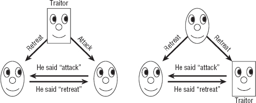
Figure 18-2: A loyal lieutenant cannot tell the difference between a traitor general and a traitor lieutenant.
In the situation on the left, the general is a traitor and gives conflicting instructions to his lieutenants, who honestly report their orders to each other.
In the situation on the right, the general is loyal and tells both lieutenants to retreat, but the lieutenant on the right lies about his orders.
In both of these cases, the lieutenant on the left sees the same result—an order to retreat from the general, and an order to attack from the other lieutenant. He doesn't know which order is true.
If there are at least three lieutenants (four people in all) and only one traitor, a simple solution exists:
- The general sends orders to the lieutenants.
- Each lieutenant tells the others what order he received from the general.
- Each lieutenant takes as his action whatever order is in the majority of those he has heard about (including the one he received from the general).
To see why this works, look at Figure 18-3. If the general is a traitor, as shown on the left, he can give conflicting orders to the lieutenants. In that case, all the lieutenants are loyal, so they faithfully report the orders they receive. That means all the lieutenants get the same information about the orders they received, so they all come to the same conclusion about which order is in the majority. For the situation on the left in Figure 18-3, all three lieutenants see two orders to attack and one order to retreat, so they all decide to attack. They arrive at a common decision, and it matches the loyal general's actual order.
If a lieutenant is a traitor, as shown on the right in Figure 18-3, the general gives all the lieutenants the same order. The traitor can report conflicting or incorrect orders to the other lieutenants to try to confuse the issue. However, the two other lieutenants receive the same order (because the general is loyal) and faithfully report their identical order. Depending on what the traitor reports, the other two lieutenants may not receive the same set of reported orders, but there are enough loyal lieutenants to guarantee that the true order is the majority decision for every lieutenant.
NOTE The majority vote solution to the general and lieutenants problem works if there are T traitors as long as there are at least 3 × T lieutenants.
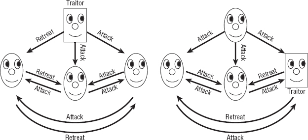
Figure 18-3: Three lieutenants can agree on a common decision no matter who the traitor is.
After you understand how to solve the general and lieutenants problem, you can reduce the byzantine generals problem to it. Assuming that each of the generals has a value Vi, the following steps give all the loyal generals the true values of the other loyal generals:
- For each general Gi:
- Run the general and lieutenants algorithm with Gi acting as the commanding general, the other generals acting as the lieutenants, and the value Gi acting as the commanding general's order.
- Each of the noncommanding generals should use the majority vote as the value Vi for general Gi.
After all the rounds of Step 1, each general knows the values owned by all the loyal generals. They may have different ideas about the values held by the traitors, but that's not a requirement of the problem.
Consensus
In the consensus problem, a number of processes must agree on a data value even if some of the processes fail. (This is very similar to the byzantine generals problem, in which the generals must agree on a plan of action even if there are traitors.) The specific rules are as follows:
- Termination—Every valid process eventually picks a value.
- Validity—If all valid processes initially propose value V, they eventually all decide on value V.
- Integrity—If a valid process decides on a value V, value V must have been proposed by some valid process.
- Agreement—All valid processes must agree on the same value in the end.
The “phase king” algorithm solves the consensus problem if up to F processes fail and there is a total of at least 4 × F + 1 processes. For example, to tolerate one failure, the algorithm requires at least five processes.
Suppose there are N processes and up to F failures. Initially each process makes a guess as to what it thinks the final value should be. Let Vi be the guess for process Pi.
To allow up to F failures, the algorithm uses a series of F + 1 phases. During each phase, one of the processes is designated as the “phase king.” You can assign the phase king based on process ID or some other arbitrary value, as long as each phase has a different phase king.
Each of the F + 1 phases consists of two rounds. In the first round, every process tells every other process its current guess about what it thinks the value should be.
Each process examines the guesses it received, plus its own current guess, and finds the majority value. If there is no majority value, it uses some predefined default value. Let Mi be the majority value for process Pi.
In the phase's second round, the current phase king process Pk broadcasts its own majority value to all the other processes to use as a tiebreaker. Each process (including the phase king) examines its majority value Mi. If the number of times Mi appears is greater than N / 2 + F, the process updates its guess by setting Vi = Mi. If the number of times Mi appears is not greater than N / 2 + F, the process sets Vi equal to the phase king's tiebreaker value.
For example, to see how this might work in a simple case, suppose there are five processes and there could be one invalid process, but in fact all the processes are working correctly. Let the phase king in phase i be process Pi, and suppose the processes' initial guesses are attack, retreat, retreat, attack, and attack, respectively:
- Phase 1, Round 1—The processes honestly broadcast their values to each other, so each thinks there are three votes of attack and two votes of retreat.
- Phase 1, Round 2—The phase king broadcasts its majority value attack to the other processes. Each process compares the number of times it saw the majority value (attack) to N / 2 + F. Each process saw the majority value three times. The value N / 2 + F = 5 / 2 + 1 = 3.5. Because the majority value did not occur more than 3.5 times, the processes all set their guesses to the tiebreaker value attack.
- Phase 2, Round 1—The processes honestly broadcast their values to each other again. Now all of them vote attack.
- Phase 2, Round 2—The phase king broadcasts its majority value attack to the other processes. This time each process sees the majority value five times. The value 5 is greater than 3.5, so each process accepts this as its guess.
Because this example tolerates up to one failure, it finishes after only two phases. In this example, every process votes to attack, which happens to be the true majority vote.
For a more complicated example, suppose there are five processes, as before, but the first fails in a byzantine way (it is a traitor). Suppose the initial guesses are <traitor>, attack, attack, retreat, attack. (The traitor doesn't have an initial guess. He just wants to mess up the others.)
- Phase 1, Round 1—In this phase, the phase king is the traitor process P1. The processes broadcast their values to each other. The traitor tells each process that it agrees with whatever that process's guess is, so the processes receive these votes:
- P1—<The traitor doesn't really care.>
- P2—Attack, attack, attack, retreat, attack
- P3—Attack, attack, attack, retreat, attack
- P4—Retreat, attack, attack, retreat, attack
- P5—Attack, attack, attack, retreat, attack
The majority votes and their numbers of occurrence for the processes are <traitor>, attack × 4, attack × 4, attack × 3, and attack × 4.
- Phase 1, Round 2—The phase king (the traitor) gives the other processes conflicting tiebreaker values. It tells P2 and P3 that the tiebreaker is attack, and it tells P4 and P5 that the tiebreaker is retreat. Processes P2, P3, and P5 see the majority value attack four times, so they accept it as their updated guess. Process P4 sees the majority value only three times. This is less than the 3.5 times required for certainty, so P4 uses the tiebreaker value retreat. The processes' new guesses are <traitor>, attack, attack, retreat, attack.
- Phase 2, Round 1—In this phase, the phase king is the valid process P2. The processes broadcast their values to each other. In a last-ditch attempt to confuse the issue, the traitor tells all the other processes that it thinks they should retreat, so the processes receive these votes:
- P1—<The traitor doesn't really care.>
- P2—Retreat, attack, attack, retreat, attack
- P3—Retreat, attack, attack, retreat, attack
- P4—Retreat, attack, attack, retreat, attack
- P5—Retreat, attack, attack, retreat, attack
The majority votes and their numbers of occurrence for the processes are <traitor>, attack × 3, attack × 3, attack × 3, and attack × 3.
- Phase 2, Round 2—The majority value for the phase king P2 is attack (seen three times), so it tells all the other processes that the tiebreaker value is attack. All the valid processes (including the phase king) see the majority value attack less than 3.5 times, so they all go with the tiebreaker value, which is attack.
At this point, all the value processes have attack as their current guess.
The reason this algorithm works is that it runs for F + 1 phases. If there are at most F failures, at least one of the phases has an honest phase king.
During that phase, suppose valid process Pi doesn't see its majority value more than N / 2 + F times. In that case, it uses the phase king's tiebreaker value.
That means all valid processes Pi that don't see a value more than N / 2 + F times end up using the same value. But what if some valid process Pj does see a value more than N / 2 + F times? Because there are at most F invalid processes, those more than N / 2 + F occurrences include more than N / 2 valid occurrences. That means there is a true majority for that value, so every process that sees a majority value more than N / 2 + F times must be seeing the same majority value. Because in this situation there is a true majority value, the current phase king must see that value as its majority value (even if the phase king doesn't necessarily see it more than N / 2 + F times).
This means that after the honest phase king's reign, all the valid processes vote for the same value.
After that point, it doesn't matter what an invalid phase king tries to do. At this point, the N − F valid processes all agree on a value. Because F < N / 4, the number of valid processes is N − F > N − (N / 4) = 3 / 4 × N = N / 2 + N / 4. Because N / 4 > F, this value is N / 2 + N / 4 > N / 2 + F. But if a valid process sees more than this number of agreeing guesses, it uses that value for its updated guess. This means all the valid processes keep their values, no matter what an invalid phase king does to try to confuse them.
Leader Election
Sometimes a collection of processes may need a central leader to coordinate actions. If the leader crashes or the network connection to the leader fails, the group must somehow elect a new leader.
The bully algorithm uses the processes' IDs to elect a new leader. The process with the largest ID wins.
Despite this simple description, the full bully algorithm isn't quite as simple as you might think. It must handle some odd situations that may arise if the network fails in various ways. For example, suppose one process declares itself the leader, and then another process with a lower ID also declares itself the leader. The first process with the higher ID should be the leader, but obviously the other processes didn't get the message.
The following steps describe the full bully algorithm:
- If process P decides the current leader has failed (because the leader has exceeded a timeout), it broadcasts an “Are you alive?” message to all processes with a larger ID.
- If process P does not receive an “I am alive” message from any process with a higher ID within a certain timeout period, process P becomes the leader by sending an “I am the leader” message to all processes.
- If process P does receive an “I am alive” message from a process with a higher ID, it waits for an “I am the leader” message from that process. If P doesn't receive that message within a certain timeout period, it assumes that the presumptive leader has failed and starts a new election from Step 1.
- If P receives an “Are you alive” message from a process with a lower ID, it replies with “I am alive” and then starts a new election from Step 1.
- If P receives an “I am the leader” message from a process with a lower ID, it starts a new election from Step 1.
In Step 5, when a lower ID process says it's the leader, the higher ID process basically says, “No, you're not,” pushes aside the lower ID process, and assumes command. This is the behavior that gives the bully algorithm its name.
Snapshot
Suppose you have a collection of distributed processes, and you want to take a snapshot of the entire system's state that represents what each process is doing at a given moment.
Actually, the timing of when the snapshot is taken is a bit hard to pin down. Suppose process A sends a message to process B, and that message is currently in transit. Should the system's state be taken before the message was sent, while the message is in transit, or after the message arrives?
You might want to try to save the system's state before the message was sent. Unfortunately, process A may not remember what its state was at that time, so this won't work (unless you require all processes to remember their past states, which could be quite a burden).
If you store only the processes' states while a message is in transit, the processes' states may be inconsistent. For example, suppose you want to restore the system's state by resetting all the processes' states to their saved states. This doesn't really restore the entire system, because the first time around, process B received the message shortly after the snapshot was taken, and that won't happen in the restored version.
For a concrete example, suppose processes A and B store the bank balances for customers A and B. Now suppose customer A wants to transfer $100 to customer B. Process A subtracts the money and sends a message to process B, telling it to add $100 to customer B's account. While the message is in transit, you take a snapshot of the system. If you later restore the system from the snapshot, customer A has already sent the $100, but customer B has not yet received it, so the $100 is lost. (This would be a terrible way to manage bank accounts. If a network failure makes a message disappear, the money also will be lost. You need to use a more secure consensus protocol to make sure both processes agree that the money has been transferred.)
So to take a good snapshot of the system, you need to save not only each process's state, but also any messages that are traveling among the processes.
The following steps describe a snapshot algorithm developed by K. Mani Chandy and Leslie Lamport:
- Any process (called the observer) can start the snapshot process. To start a snapshot:
- The observer saves its own state.
- The observer sends a snapshot message to all other processes. The message contains the observer's address and a snapshot token that indicates which snapshot this is.
- If a process receives a particular snapshot token for the first time:
- It sends the observer its saved state.
- It attaches a snapshot token to all subsequent messages that it sends to any other process.
- Suppose process B receives the snapshot token and then later receives a message from process A that does not have the snapshot token attached. In that case, the message was in transit. It was sent before process A received the snapshot token, so it is not taken into account by process A's saved state. To make sure this information isn't lost, process B sends a copy of the message to the observer.
After all the messages have finished flowing through the system, the observer has a record of every process's state and of any messages that were in transit when the snapshot was taken.
Clock Synchronization
Exact clock synchronization can be tricky due to inconsistent message transmission times that occur in a shared network. The problem becomes much easier if processes communicate directly without using a network. For example, if two computers are in the same room and you connect them with a wire, you can measure the wire's length, calculate the time it takes for a signal to travel across the wire, and then use it to synchronize the computers' clocks.
This works, but it is cumbersome and may not be possible between computers that are far apart. Fortunately, you can synchronize two processes' clocks fairly well by using a network if you assume that a network's message transmission time doesn't vary too much over a short period of time.
Suppose you want process B to synchronize its clock to the clock used by process A. Call the time according to process A the “true” time.
The following steps describe the messages the processes should exchange:
- Process A sends process B a message containing TA1 (the current time according to process A).
- Process B receives the message and sends process A a reply containing TA1 and TB1 (the current time according to process B).
- Process A receives the reply and sends process B a new message containing TA1, TB1, and TA2 (the new current time according to process A).
Now process B can perform some calculations to synchronize its clock with process A.
Suppose E is the error between the two clocks, so TB = TA + E at any given time. Also suppose D is the delay required to send a message between the two processes.
When process B records time TB1, the initial message took time D to get from process A to process B, so:
![]()
Similarly, when process A records time TA2, the reply took time D to get from process B to process A, so:
![]()
If you subtract the second equation from the first, you get:
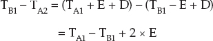
Solving this equation for E gives:
![]()
Now process B has an estimate of E, so it can adjust its clock accordingly.
This algorithm assumes that the delay remains roughly constant during the time it takes to pass the messages back and forth. It also assumes that a message from A to B takes about the same amount of time as a message from B to A.
Summary
This chapter has discussed issues that involve parallel processing. It explained some of the different models of parallel computation and described several algorithms that run in distributed systems. You may not need to use some of the more esoteric algorithms, such as the zero-time sort on a systolic array or the solution to the dining philosophers problem, but all these algorithms highlight some of the problems that can arise in distributed systems. Those problems include such issues as race conditions, deadlock, livelock, consistency, and synchronization.
Distributed environments range from desktop and laptop computers with multiple cores to huge grid projects that use hundreds of thousands of computers to attack a single problem. Even if Moore's Law holds for another decade or two, so much underused processing power already is available that it makes sense to try to take advantage of it with distributed computing. To get the most out of today's computing environments and the increasingly parallel environments that are on their way, you must be aware of these issues and the approaches that you can use to solve them.
Exercises
Asterisks indicate particularly difficult problems.
- Make a diagram similar to the one shown in Figure 18-1, showing how the zero-time sorting algorithm would sort the two lists 3, 5, 4, 1 and 7, 9, 6, 8 simultaneously. Draw one set of numbers bold or in a different color to make it easier to keep the two lists separate as the algorithm runs. How many more ticks are required to sort the two lists instead of just one?
- In many systems, a process can safely read a shared memory location, so it only needs a mutex to safely write to the location. (The system is said to have atomic reads, because a read operation cannot be interrupted in the middle.) What happens to the Hamiltonian path example if the process reads the shared total route length in the If statement and then acquires the mutex as its first statement inside the If Then block?
- *Consider the Chandy/Misra solution to the dining philosophers problem. Suppose the philosophers are synchronized, and suppose they all immediately attempt to eat. Assume that a philosopher thinks for a long time after eating, so none of them needs to eat a second time before the others have eaten.
In what order do the philosophers eat? In other words, who eats first, second, third, and so on? (Hint: It may be helpful to draw a series of pictures to show what happens.)
- In the two generals problem, what happens if some of the initial messages get through, and general B sends some acknowledgments, but he is unlucky, and none of the acknowledgments makes it back to general A?
- In the two generals problem, let PAB be the probability that a messenger is caught going from general A to general B. Let PBA be the probability that a messenger is caught going from general B to general A. The original algorithm assumes that PAB = PBA, but suppose that isn't true. How can the generals figure out the two probabilities?
- Consider the three-person general and lieutenant problem shown in Figure 18-2. You could try to solve the problem by making a rule that any lieutenant who hears conflicting orders should follow the order given by the general. Why won't that work?
- Consider the three-person general and lieutenant problem shown in Figure 18-2. You could try to solve the problem by making a rule that any lieutenant who hears conflicting orders should retreat. Why won't that work?
- In the four-person general and lieutenant problem shown in Figure 18-3, can the loyal lieutenants figure out who the traitor is? If they cannot, how many lieutenants would be needed to figure it out?
- In the four-person general and lieutenant problem shown in Figure 18-3, find a scenario that allows the lieutenants to identify the traitor. In that scenario, what action should the lieutenants take? (Of course, if the traitor is smart, he will never let this happen.)
- What modification would you need to make to the dining philosophers problem to let the leader algorithm help with it? How would it help?
- Would a bully-style algorithm help with the dining philosophers problem?
- Define a ravenous philosophers problem. It is similar to the dining philosophers problem, except this time the philosophers are always hungry. After a philosopher finishes eating, he puts down his forks. If no one picks them up right away, he grabs them and eats again. What problems would this cause? What sort of algorithm might fix the problems?
- In the clock synchronization algorithm, suppose the time needed to send a message from A to B differs from the time needed to send a message from B to A. How much error could this difference introduce into the final value for process B's clock?
- The clock synchronization algorithm assumes that message-sending times are roughly constant during the message exchange. If the network's speed changes during the algorithm, how much error could that introduce into the final value for process B's clock?
- Suppose a network's speed varies widely over time. How could you use the answer to Exercise 14 to improve the clock synchronization algorithm?