
Chapter 18
Portfolio Insurance: The Extreme Value Approach Applied to the CPPI Method
Philippe Bertrand1,2 and Jean-Luc Prigent3
1CERGAM, Aix-Marseille University, Aix, France
2KEDGE Business School, Marseille, France
3THEMA and Labex MME-DII, University of Cergy-Pontoise, Cergy-Pontoise, France
18.1 Introduction
Portfolio insurance is designed to give the investor the ability to limit downside risk while allowing some participation in upside markets. This return pattern has seemed attractive to many investors who have poured up to billions of dollars into various portfolio insurance products, based either on basic financial assets such as equity or bond indices or on more complex assets such as credit products and hedge funds. There exist several methods of portfolio insurance: stop-loss strategy, the option-based portfolio insurance (OBPI) introduced by Leland and Rubinstein (1976), the constant proportion portfolio insurance (CPPI), and so on (see Bertrand and Prigent, 2005 for a comparison of these methods).
Here, we are interested in a widely used one: the CPPI introduced by Black and Jones (1987) for equity instruments and by Perold (1986) and Perold and Sharpe (1988) for fixed-income instruments (see also Black and Perold, 1992). The standard CPPI method uses a simplified strategy to allocate assets dynamically over time. It requires that two assets are exchanged on the financial market: the riskless asset with a constant interest rate (usually treasury bills or other liquid money market instruments), and the risky one (usually a market index or a basket of market indices). The key assumption is that, at any time of the management period, the amount invested on the risky asset (usually called the exposure) is proportional to the difference (usually called the cushion) between the current portfolio value and the floor, which corresponds to the guaranteed amount. In particular, such a method implies (theoretically) that the exposure is nil as soon as the cushion is nil. Advantages of this strategy over other approaches to portfolio insurance are its simplicity and its flexibility. The initial cushion and the floor can be chosen according to the own investor's objective, while the multiple can be derived from the maximization of the expected utility of the investor (see Prigent, 2001a). However, in that case, the optimal multiple may be a function of the risky asset, as shown in El Karoui et al. (2005). Usually, banks do not directly bear market risks on the asset portfolios they manage for their customers. This is not necessarily true when we consider management of insured portfolios. In that case, banks can use, for example, stress testing since they may suffer the consequences of sudden large market decreases, depending on their management method.1 For instance, in the case of the CPPI method, banks must at least provision the difference on their own capital if the value of the portfolio drops below the floor. Therefore, one crucial question for the bank that promotes such funds is: what exposure to the risky asset or, equivalently, what level of the multiple to accept? On one hand, as portfolio expectation return is increasing with respect to the multiple, customers want the multiple as high as possible. On the other hand, due to market imperfections,2 portfolio managers must impose an upper bound on the multiple m. First, if the portfolio manager anticipates that the maximum daily historical drop (e.g., −20%) will happen during the period, he chooses m smaller than 5, which leads to a low return expectation. Alternatively, he may think that the maximum daily drop during the period he manages the portfolio will never be higher than a given value (e.g., −10%). A straightforward implication is to choose m according to this new extreme value (e.g., ![]() ). Another possibility is that, more accurately, he takes account of the occurrence probabilities of extreme events in the risky asset returns. Finally, he can adopt a quantile hedging strategy: choose the multiple as high as possible but so that the portfolio value will always be above the floor at a given probability level (typically 99%). However, he must take care of heavy tails in the return distribution, as emphasized in Longin (2000) and also in Hyung and De Vries (2007). The answer to the previous questions has important practical implications in the management process implementation. It is addressed in this chapter, using extreme value theory (EVT).
). Another possibility is that, more accurately, he takes account of the occurrence probabilities of extreme events in the risky asset returns. Finally, he can adopt a quantile hedging strategy: choose the multiple as high as possible but so that the portfolio value will always be above the floor at a given probability level (typically 99%). However, he must take care of heavy tails in the return distribution, as emphasized in Longin (2000) and also in Hyung and De Vries (2007). The answer to the previous questions has important practical implications in the management process implementation. It is addressed in this chapter, using extreme value theory (EVT).
This chapter is organized as follows. Section 18.2 presents the model and its basic properties. In Section 18.3, we examine the gap risk of the CPPI method and provide upper bounds on the multiple, in particular when using a quantile hedging approach. EVT allows us to get approximation of these bounds. We provide an empirical illustration using S&P 500 data.
18.2 The CPPI Method
18.2.1 Illustrative Example
To illustrate the method (see Figure 18.1), consider, for example, an investor with initial amount to invest ![]() (=100). Assume the investor wants to recover a prespecified percentage
(=100). Assume the investor wants to recover a prespecified percentage ![]() (= 95%) of her initial investment at a given date in the future, T (=1 year). Note that the insured terminal value
(= 95%) of her initial investment at a given date in the future, T (=1 year). Note that the insured terminal value ![]() (=95) cannot be higher than the initial value capitalized at the risk-free rate (= 3%),
(=95) cannot be higher than the initial value capitalized at the risk-free rate (= 3%), ![]() (= 103.04). Her portfolio manager starts by setting an initial floor
(= 103.04). Her portfolio manager starts by setting an initial floor ![]() (= 92.2). To get a portfolio value
(= 92.2). To get a portfolio value ![]() at maturity t higher than the insured amount
at maturity t higher than the insured amount ![]() , he keeps the portfolio value
, he keeps the portfolio value ![]() above the floor
above the floor ![]() at any time t during the management period
at any time t during the management period ![]() . For this purpose, the amount
. For this purpose, the amount ![]() invested in the risky asset is a fixed proportion m of the excess
invested in the risky asset is a fixed proportion m of the excess ![]() of the portfolio value over the floor. The constant m is usually called the multiple,
of the portfolio value over the floor. The constant m is usually called the multiple, ![]() the exposure, and
the exposure, and ![]() the cushion. Since
the cushion. Since ![]() , this insurance method consists in keeping
, this insurance method consists in keeping ![]() positive at any time t in the period. The remaining funds are invested in the riskless asset
positive at any time t in the period. The remaining funds are invested in the riskless asset ![]() .
.
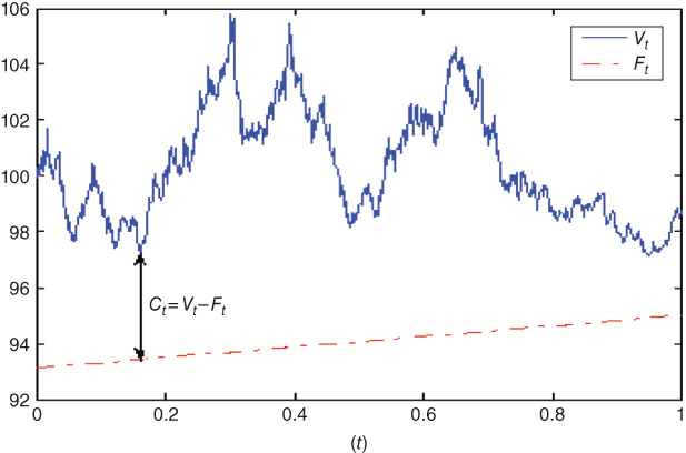
Figure 18.1 The CPPI method.
Both the floor and the multiple are functions of the investor's risk tolerance. The higher the multiple, the more the investor will participate in a sustained increase in stock prices. Nevertheless, the higher the multiple, the faster the portfolio will approach the floor when there is a sustained decrease in stock prices. As the cushion approaches zero, exposure approaches zero, too. Normally, this keeps the portfolio value from falling below the floor. Nevertheless, during financial crises, a very sharp drop in the market may occur before the manager has a chance to trade. This implies that m must not be too high (e.g., if a fall of 10% occurs, m must not be higher than 10 in order to keep the cushion positive).
18.2.2 The CPPI Method (Continuous-Time Case)
The continuous-time framework is generally introduced to study the CPPI method as in Perold (1986). Recall that it is based on a dynamic portfolio strategy so that the portfolio value is above a floor F at any time t. The value of the floor gives the dynamical insured amount. It is assumed to evolve as a riskless asset, according to
Obviously, the initial floor ![]() is smaller than the initial portfolio value
is smaller than the initial portfolio value ![]() . The difference
. The difference ![]() is called the cushion, denoted by
is called the cushion, denoted by ![]() . Its value
. Its value ![]() at any time t in
at any time t in ![]() is given by
is given by
Denote by ![]() the exposure, which is the total amount invested in the risky asset. The standard CPPI method consists of letting
the exposure, which is the total amount invested in the risky asset. The standard CPPI method consists of letting
where m is a constant called the multiple.
Note that the interesting case for portfolio insurance corresponds to ![]() . When the risky asset dynamics follows a geometric Brownian motion, it implies that the portfolio value at maturity is a convex function of the risky asset value. Such feature can provide significant percentage of the market rise.
. When the risky asset dynamics follows a geometric Brownian motion, it implies that the portfolio value at maturity is a convex function of the risky asset value. Such feature can provide significant percentage of the market rise.
Assume that the risky asset price process ![]() is a diffusion process with jumps:
is a diffusion process with jumps:
where ![]() is a standard Brownian motion, independent of the Poisson process
is a standard Brownian motion, independent of the Poisson process ![]() that models jumps. All coefficient functions satisfy usual assumptions to guarantee the existence and uniqueness of the previous stochastic differential equation. It means, in particular, that the sequence of random times
that models jumps. All coefficient functions satisfy usual assumptions to guarantee the existence and uniqueness of the previous stochastic differential equation. It means, in particular, that the sequence of random times ![]() corresponding to jumps satisfies the following properties: the inter-arrival times
corresponding to jumps satisfies the following properties: the inter-arrival times ![]() are independent and have the same exponential distribution with parameter denoted by
are independent and have the same exponential distribution with parameter denoted by ![]() .
.
The relative jumps of the risky asset ![]() are equal to
are equal to ![]() . They are supposed to be strictly higher than −1 (in order for the price S to be nonnegative). We deduce the portfolio value and its basic properties (see Prigent, 2007).
. They are supposed to be strictly higher than −1 (in order for the price S to be nonnegative). We deduce the portfolio value and its basic properties (see Prigent, 2007).
Let us examine the Lévy process case. For this, we assume that ![]() is not equal to
is not equal to ![]() but
but ![]() and
and ![]() are constant. Suppose also that the jumps are i.i.d. with probability distribution
are constant. Suppose also that the jumps are i.i.d. with probability distribution ![]() , with finite mean
, with finite mean ![]() denoted by
denoted by ![]() and
and ![]() equal to c. The logarithmic return of the risky asset S is a Lévy process. Then, we deduce the following:
equal to c. The logarithmic return of the risky asset S is a Lévy process. Then, we deduce the following:
18.2.3 The CPPI Method (Discrete-Time Case)
Previous modeling is based on the continuous-time strategy. However, continuous-time processes are usually estimated from discrete-time observations. In that case, we have to decide whether a given return observation is due to a jump or to a relatively high fluctuation of the diffusion component (see the literature about statistical estimation of stochastic processes, and in particular, estimation of diffusion processes with jumps based on bi-power variations and its extensions). One solution is to consider that there exists a jump as soon as the observed arithmetic return lies in a given subset. However, in such a case, we have to take account of the inter-arrival time distribution.
Additionally, from the practical point of view, the discrete-time framework is more convenient since the actual CPPI strategy is based on discrete-time portfolio rebalancing. Additionally, transaction costs and/or illiquidity problems on some specific financial assets can induce discrete-time strategies.
18.2.3.1 The standard discrete-time case
Changes in asset prices are supposed to occur at discrete times along a whole time period ![]() (e.g., 10 years). Particular subperiods indexed by
(e.g., 10 years). Particular subperiods indexed by ![]() ,
, ![]() with
with ![]() , can be introduced. They may correspond to several standard portfolio management periods (e.g., 1 week, 1 month, 1 year, etc.). Finally, for each subperiod
, can be introduced. They may correspond to several standard portfolio management periods (e.g., 1 week, 1 month, 1 year, etc.). Finally, for each subperiod ![]() , consider the sequence of deterministic prices variations times
, consider the sequence of deterministic prices variations times ![]() in
in ![]() , which for simplicity, for each
, which for simplicity, for each ![]() , we denote by
, we denote by ![]() (e.g., daily variations).
(e.g., daily variations).
In this framework, the CPPI portfolio value can be determined as follows. Denote by ![]() the opposite of the arithmetical return of the risky asset between times
the opposite of the arithmetical return of the risky asset between times ![]() and
and ![]() . We have
. We have
Consider the maximum of these values. For any ![]() , define
, define
Denote by ![]() the portfolio value at time
the portfolio value at time ![]() . The guarantee constraint is to keep the portfolio value
. The guarantee constraint is to keep the portfolio value ![]() above the floor
above the floor ![]() . The exposure
. The exposure ![]() invested in the risky asset
invested in the risky asset ![]() is equal to
is equal to ![]() , where the cushion value
, where the cushion value ![]() is equal to
is equal to ![]() . The remaining amount
. The remaining amount ![]() is invested on the riskless asset with return
is invested on the riskless asset with return ![]() for the time period
for the time period ![]() . Therefore, the dynamic evolution of the portfolio value is given by (similar to the continuous-time case)
. Therefore, the dynamic evolution of the portfolio value is given by (similar to the continuous-time case)
where the cushion value is defined by
Thus, we deduce both the cushion and the portfolio values.
For example, if the maximum drop is equal to −20% (the “Black Monday” on October 1987), then d = −0.2. Thus m must be less than 5.
18.2.3.2 The “truncated” discrete-time case
Because of the discrete-time estimation of stochastic processes or of the possible anticipation of the portfolio manager concerning the relative jumps during a given period (e.g., ![]() is considered as an actual jump if its value is higher than 3% or
is considered as an actual jump if its value is higher than 3% or ![]() will never be higher than 20%, corresponding to the market crash in October 1987), we introduce also the truncated jumps
will never be higher than 20%, corresponding to the market crash in October 1987), we introduce also the truncated jumps ![]() defined by
defined by
where ![]() is equal to 1 if
is equal to 1 if ![]() , and 0 otherwise.
, and 0 otherwise.
In fact, when determining an upper bound on the multiple m, we have only to consider positive values of ![]() (see Section 18.3). Therefore, it is sufficient to take
(see Section 18.3). Therefore, it is sufficient to take ![]() and
and ![]() equal to the maximum relative drop anticipated for the management period. Since the portfolio manager may take account of the occurrence probabilities of some given values of the relative jumps (corresponding, e.g., to maximum drops), we must introduce their arrival times which are random variables. Denote by
equal to the maximum relative drop anticipated for the management period. Since the portfolio manager may take account of the occurrence probabilities of some given values of the relative jumps (corresponding, e.g., to maximum drops), we must introduce their arrival times which are random variables. Denote by ![]() the sequence of times at which
the sequence of times at which ![]() takes values in the interval
takes values in the interval ![]() . The sequence
. The sequence ![]() is called a marked point process.3
is called a marked point process.3
18.3 CPPI and Quantile Hedging
18.3.1 Upper Bounds on the Multiple
As seen in Proposition 18.4, there exists an upper bound on the multiple, which allows the perfect guarantee. However, this latter one is usually rather stringent and does not allow making significant benefit from market rises.
This strong condition can be modified if a quantile hedging approach is adopted, like the value at risk (see Föllmer and Leukert, 1999 for application of this notion in financial modeling). This gives the following relation for a time period ![]() :
:
18.3.1.1 The standard discrete-time case
In our framework, the portfolio manager must keep the cushion positive for each trading day. Thus, we measure stock market price fluctuations by the daily rates of returns. More precisely, we use the opposite of the arithmetical rate ![]() , which determines the conditions to impose on the multiple m, within the context of the CPPI method. If these variables are statistically independent and drawn from the same distribution, then the exact distribution of the maximum is equal to the power of the common distribution of
, which determines the conditions to impose on the multiple m, within the context of the CPPI method. If these variables are statistically independent and drawn from the same distribution, then the exact distribution of the maximum is equal to the power of the common distribution of ![]() .
.
Assume that the random variables ![]() are not truncated and the arrival times are the times
are not truncated and the arrival times are the times ![]() themselves. Let us consider
themselves. Let us consider ![]() the maximum of the
the maximum of the ![]() for all times
for all times ![]() in
in ![]() . Then, the previous quantile condition is equivalent to
. Then, the previous quantile condition is equivalent to
Note that, since m is nonnegative, the condition ![]() is equivalent to
is equivalent to ![]() .
.
If the N random variables ![]() are i.i.d. with cumulative distribution function (CDF) F, then we get the following result:
are i.i.d. with cumulative distribution function (CDF) F, then we get the following result:
But, in most cases the CDF F is not exactly known, and some consecutive returns can be dependent. However, if block-maxima can be assumed to be independent by using a suitable length of the blocks, then the insurance condition on the multiple m can be analyzed by applying EVT.
Indeed, the fundamental result of EVT proves that there exists a normalization procedure of the maxima to get nondegenerate distributions at the limit (like the well-known central limit theorem for the sums of random variables).4 This is the well-known Fisher–Tippett theorem (1928). Indeed, we know that there exist scale and location parameters ![]() and
and ![]() such that
such that ![]() converges in distribution to a generalized extreme distributions (GEV) defined by
converges in distribution to a generalized extreme distributions (GEV) defined by

where the parameter ![]() is called the tail index:
is called the tail index:

Consequently, from the condition ![]() , and by applying EVT to
, and by applying EVT to ![]() , we get
, we get ![]() . This leads to the result. Indeed, we get the following approximation of the upper limit on multiple m.
. This leads to the result. Indeed, we get the following approximation of the upper limit on multiple m.
The statistical problem is to find the correct distribution of extremes of returns from the data and, in particular, to estimate the normalizing constants ![]() , and the tail index
, and the tail index ![]() . For this purpose, when using a maximum likelihood method, we need the GEV distribution of a general, non-centered, non-reduced random variable, defined by
. For this purpose, when using a maximum likelihood method, we need the GEV distribution of a general, non-centered, non-reduced random variable, defined by

When examining the sequence ![]() , it is obvious that its distribution has a right end limit equal to 1. Therefore, the normalized maxima
, it is obvious that its distribution has a right end limit equal to 1. Therefore, the normalized maxima ![]() converge either to the Gumbel distribution
converge either to the Gumbel distribution ![]() or to a Weibull distribution
or to a Weibull distribution ![]() . For the sequence of the opposite of log-returns
. For the sequence of the opposite of log-returns ![]() , we get a Gumbel distribution or a Fréchet distribution.
, we get a Gumbel distribution or a Fréchet distribution.
For the determination of the limit, we can use the characterizations of Resnik (1987) for the maximum domains of attraction based on generalizations of the von Mises functions (see Embrechts et al., 1997).
18.3.1.2 The “truncated” discrete-time case
Consider now the truncated values ![]() ; denote the truncated jumps (
; denote the truncated jumps (![]() ), and
), and ![]() the corresponding sequence of arrival times. As has been previously mentioned, the times
the corresponding sequence of arrival times. As has been previously mentioned, the times ![]() are random variables and the range of their distributions can be the set of times
are random variables and the range of their distributions can be the set of times ![]() or the whole management period
or the whole management period ![]() if we consider jump-diffusion processes.
if we consider jump-diffusion processes.
Define ![]() as the maximum of the
as the maximum of the ![]() in
in ![]() . The quantile hedging condition leads to
. The quantile hedging condition leads to
Denote by ![]() the random number of random variables
the random number of random variables ![]() during the period
during the period ![]() .
.
Then, by conditioning with respect to the random number ![]() , the quantile hedging condition becomes
, the quantile hedging condition becomes
which is equivalent to
Introduce the function ![]()
Since ![]() is increasing,
is increasing, ![]() has also the same property. Consider its inverse
has also the same property. Consider its inverse ![]() .
.
Then we get the following result:
As can be seen, this condition involves the joint conditional distributions of the marked point process ![]() . In the independent marking case, where
. In the independent marking case, where ![]() and
and ![]() are independent, the CDF
are independent, the CDF ![]() can be simplified as
can be simplified as
Suppose, for example, that the number of times ![]() is sufficiently high so that we can consider that the set of
is sufficiently high so that we can consider that the set of ![]() seems like an interval (continuous time at the limit). Assume also that the sequence of inter-arrival times
seems like an interval (continuous time at the limit). Assume also that the sequence of inter-arrival times ![]() is an i.i.d. sequence and is exponentially distributed with a parameter
is an i.i.d. sequence and is exponentially distributed with a parameter ![]() . This case corresponds to the special case of an independent marked Poisson process.
. This case corresponds to the special case of an independent marked Poisson process. ![]() corresponds also to the parameter of the Poisson counting distribution. This implies that the expectation of the number of variations with values in
corresponds also to the parameter of the Poisson counting distribution. This implies that the expectation of the number of variations with values in ![]() during the period
during the period ![]() is equal to
is equal to ![]() . We get
. We get
Furthermore, if ![]() are also i.i.d., then we get (see Prigent, 2001b)
are also i.i.d., then we get (see Prigent, 2001b)
This latter formula allows the explicit calculation of the upper bound.
This condition gives an upper limit on the multiple m, which is obviously greater than the standard limit ![]() (which is given in Proposition 18.4 with b = d if the distribution is not truncated). It takes account of both the distribution of the variations and of the inter-arrival times. Note that, if the intensity
(which is given in Proposition 18.4 with b = d if the distribution is not truncated). It takes account of both the distribution of the variations and of the inter-arrival times. Note that, if the intensity ![]() increases, then this upper limit decreases. So, as intuition suggests, if the frequency
increases, then this upper limit decreases. So, as intuition suggests, if the frequency ![]() increases, then the multiple has to be reduced and, if
increases, then the multiple has to be reduced and, if ![]() goes to infinity, then the previous upper limit converges to the standard limit
goes to infinity, then the previous upper limit converges to the standard limit ![]() .
.
Again, if the distribution of the opposite of arithmetic returns is not known, we can apply EVT to get approximation of the upper bound, provided that the management period ![]() over which the risk is evaluated is sufficiently high and that the probabilities
over which the risk is evaluated is sufficiently high and that the probabilities ![]() are small, for small values of k. Under the previous conditions, we get
are small, for small values of k. Under the previous conditions, we get

From the practical point of view, condition “![]() small, for small values of k” implies that the set
small, for small values of k” implies that the set ![]() is not too small. Thus, we have to carefully calibrate this set in order to get rational upper bounds.
is not too small. Thus, we have to carefully calibrate this set in order to get rational upper bounds.
18.3.2 Empirical Estimations
In what follows, we illustrate numerically the upper bound given in Proposition 18.10 when dealing with upper bound for block-maxima series.
18.3.2.1 Estimations of the variations Xk
We examine the variations of the opposite of the arithmetic returns, ![]() , of the S&P 500 during both the period December 1983–December 2013 and the subperiod December 2003–December 2013. First we consider the whole support of
, of the S&P 500 during both the period December 1983–December 2013 and the subperiod December 2003–December 2013. First we consider the whole support of ![]() . We refer to Longin (1996b) for details about estimation procedures when dealing with EVT. We begin with some usual descriptive statistics about daily variations
. We refer to Longin (1996b) for details about estimation procedures when dealing with EVT. We begin with some usual descriptive statistics about daily variations ![]() (Table 18.1).
(Table 18.1).
Table 18.1 Descriptive statistics of daily variations
| S&P 500 (10 years) | S&P 500 (30 years) | |
| Mean | −0.029057% | −0.038591% |
| Median | −0.078802% | −0.056489% |
| Maximum | 0.0903 | 0.2047 |
| Minimum | −0.1158 | −0.1459 |
| Standard deviation | 0.0129 | 0.0116 |
| Skewness | 0.0762 | 0.5550 |
| Kurtosis | 14.3041 | 27.0027 |
| Jarque-Bera | 13409 | 18040 |
As expected, ![]() is far from normally distributed and has fat tails. We find evidence for heteroskedasticity and autocorrelation in the series. More precisely, the original series should be replaced by the innovation of an AR(5).5 Nevertheless, the estimates on the raw data do not differ qualitatively from the ones on innovations.6 As we need estimates on the raw data for the upper bound on the multiple, we conduct econometrics work on the original series.
is far from normally distributed and has fat tails. We find evidence for heteroskedasticity and autocorrelation in the series. More precisely, the original series should be replaced by the innovation of an AR(5).5 Nevertheless, the estimates on the raw data do not differ qualitatively from the ones on innovations.6 As we need estimates on the raw data for the upper bound on the multiple, we conduct econometrics work on the original series.
We examine the behavior of maxima for various time periods. We first plot the maxima of ![]() over 20 and 60 days for the two time periods (Figures 18.2 and 18.3).
over 20 and 60 days for the two time periods (Figures 18.2 and 18.3).


Figure 18.2 Maxima (20 days).


Figure 18.3 Maxima (60 days).
Notice, first, that on our sample the maximum values of ![]() are always positive. Knowing that we have to discriminate between the Weibull and the Gumbel distribution, the analysis confirms that the extremes of
are always positive. Knowing that we have to discriminate between the Weibull and the Gumbel distribution, the analysis confirms that the extremes of ![]() seems to follow a Weibull distribution.
seems to follow a Weibull distribution.
Equivalently, we can introduce the opposite of the log-returns:

In that case, we get a Fréchet distribution.
We consider the maximum likelihood estimation of GEV distribution of the non-normalized series (see Martins and Stedinger, 2000). The density is given by

The likelihood function to maximize is defined as follows:

The estimation results for a Fréchet distribution and for various lengths of the subperiod ![]() are reported in Table 18.2.
are reported in Table 18.2.
Table 18.2 Estimation results for a Fréchet distribution
| Length of the selection period | Tail parameter ξ | Scale parameter ψθ | Location parameter μθ |
| Estimation over 10 years | |||
| θ = 5 | 0.3210 | 0.0062 | 0.0074 |
| θ = 20 | 0.4162 | 0.0071 | 0.0134 |
| θ = 60 | 0.3704 | 0.0086 | 0.0186 |
| θ = 120 | 0.4741 | 0.0081 | 0.0227 |
| θ = 240 | 0.5589 | 0.0108 | 0.0258 |
| Estimation over 30 years | |||
| θ = 5 | 0.2296 | 0.0059 | 0.0071 |
| θ = 20 | 0.2936 | 0.0068 | 0.0130 |
| θ = 60 | 0.3816 | 0.0079 | 0.0186 |
| θ = 120 | 0.4614 | 0.0098 | 0.0221 |
| θ = 240 | 0.4978 | 0.0142 | 0.0287 |
18.3.2.2 Estimations of the upper bound
We are now able to give an estimation of the upper bound on the multiple. From Proposition 18.10, the upper bound is given by ![]() , where
, where ![]() denotes the number of transaction dates during the management period. For the log-returns, we get an analogous expression of the upper bound:
denotes the number of transaction dates during the management period. For the log-returns, we get an analogous expression of the upper bound:

where ![]() denotes the inverse of the extreme distribution of maxima of
denotes the inverse of the extreme distribution of maxima of ![]() .
.
We illustrate numerically this upper bound in Table 18.3.
Table 18.3 Numerical upper bounds on the multiple
| Length of the selection period | ϵ = 5% | ϵ = 1% | ϵ = 0.1% |
| Estimation over 10 years | |||
| θ = 5 | 23.8 | 12.4 | 5.6 |
| θ = 20 | 18.6 | 9.4 | 3.9 |
| θ = 60 | 12.2 | 5.7 | 2.4 |
| θ = 120 | 7 | 3.1 | 1.4 |
| θ = 240 | 5.3 | 2.3 | 1.1 |
| Estimation over 30 years | |||
| θ = 5 | 28.2 | 16.1 | 8.4 |
| θ = 20 | 22.6 | 13.1 | 6.5 |
| θ = 60 | 15.1 | 8 | 3.8 |
| θ = 120 | 7.1 | 3.3 | 1.5 |
| θ = 240 | 5.3 | 2.4 | 1.2 |
As expected, the upper bound on the multiple decreases when the probability level ![]() decreases, which corresponds to a more stringent gap risk control. It also decreases when the length of the selection period
decreases, which corresponds to a more stringent gap risk control. It also decreases when the length of the selection period ![]() increases because at the same time the risk of significant drops increases. If bank “risk tolerance” to the probability level is very small, say
increases because at the same time the risk of significant drops increases. If bank “risk tolerance” to the probability level is very small, say ![]() , while the length of the rebalancing period is short, or if the length of the rebalancing period is high with
, while the length of the rebalancing period is short, or if the length of the rebalancing period is high with ![]() , the upper bound on the multiple is in line with standard values of the multiple used by practitioners (between 4 and 8). As soon as bank risk tolerance is higher,
, the upper bound on the multiple is in line with standard values of the multiple used by practitioners (between 4 and 8). As soon as bank risk tolerance is higher, ![]() , the corresponding multiple is above its usual values except for long periods. Note also that the upper bounds on the multiple are smaller when dealing with data on the past 10 years due to the more important impact of the financial crisis than for the longer time period corresponding to 30 years. However, for long management period (e.g., 1 year corresponding to
, the corresponding multiple is above its usual values except for long periods. Note also that the upper bounds on the multiple are smaller when dealing with data on the past 10 years due to the more important impact of the financial crisis than for the longer time period corresponding to 30 years. However, for long management period (e.g., 1 year corresponding to ![]() trading days) and for
trading days) and for ![]() (resp.
(resp. ![]() ), the upper bound is small (resp. very small) compared to m = 5, which corresponds to the historical maximum daily drop of about 20%. In fact, when using the Fréchet distribution with parameter values in Table 18.3 for
), the upper bound is small (resp. very small) compared to m = 5, which corresponds to the historical maximum daily drop of about 20%. In fact, when using the Fréchet distribution with parameter values in Table 18.3 for ![]() , we can check that the probability that the maximum daily drop is higher than 20% is about 25%, which is much higher. This is due to the weak convergence speed to the extreme distribution. On the contrary, using parameter values for the maximum on a week, this probability is much more in accordance with empirical frequency. Of course, it is possible to consider the dependence in the time series, such as the GARCH or stochastic volatility models. In that case, we can use results about the asymptotic of maxima. Note that, for example, using results of Davis and Mikosch (2009) for GARCH models, the upper bound involves the extremal index, which is the inverse of the mean cluster size of exceedances (see Ben Ameur et al., 2015). Another way to solve this problem is to introduce time-varying conditional multiples together with local quantile or expected shortfall risk measures to better take account of market fluctuations (see Ben Ameur and Prigent, 2014; Hamidi et al., 2014).
, we can check that the probability that the maximum daily drop is higher than 20% is about 25%, which is much higher. This is due to the weak convergence speed to the extreme distribution. On the contrary, using parameter values for the maximum on a week, this probability is much more in accordance with empirical frequency. Of course, it is possible to consider the dependence in the time series, such as the GARCH or stochastic volatility models. In that case, we can use results about the asymptotic of maxima. Note that, for example, using results of Davis and Mikosch (2009) for GARCH models, the upper bound involves the extremal index, which is the inverse of the mean cluster size of exceedances (see Ben Ameur et al., 2015). Another way to solve this problem is to introduce time-varying conditional multiples together with local quantile or expected shortfall risk measures to better take account of market fluctuations (see Ben Ameur and Prigent, 2014; Hamidi et al., 2014).
18.4 Conclusion
As expected, it is possible to choose higher multiples for the CPPI method than standard values if quantile hedging is used. The upper bounds can be calculated for each level of probability, according to the distributions of the marked point process, which indicates the variations of the underlying asset and its times of variations. EVT allows the approximation of these distributions in order to provide a numerical upper bound. We have illustrated this result on S&P 500 data. The difference with the standard multiple is significant, especially if we consider that the highest historical daily market decrease is unlikely to appear during the management period and when the probability level is not too small.
References
- Ben Ameur, H., Prigent, J.-L. Portfolio insurance: gap risk under conditional multiples. European Journal of Operational Research 2014;236:238–253.
- Ben Ameur, H., Bertrand, P., Prigent, J.-L. Extreme value theory for portfolio insurance with multiple assets. Working Paper Thema, University of Cergy-Pontoise, France; 2015.
- Bertrand, P., Prigent, J.-L. Portfolio insurance strategies: OBPI versus CPPI. Finance 2005;26:5–32.
- Black, F., Jones, R. Simplifying portfolio insurance. Journal of Portfolio Management 1987;14:48–51.
- Black, F., Perold, A.R. Theory of constant proportion portfolio insurance. Journal of Economic Dynamics and Control 1992;16:403–426.
- Bremaud, P. Point Processes and Queues: Martingale Dynamics. Berlin: Springer Verlag; 1981.
- Davis, R.A., Mikosch, T. Extreme value theory for GARCH processes. In: Andersen, T.G., Davis, R.A., Kreiss, J.-P., Mikosch, T., editors. Handbook of Financial Time Series. New York: Springer; 2009. p 187–200.
- El Karoui, N., Jeanblanc, M., Lacoste, V. Optimal portfolio management with American capital guarantees. Journal of Economic Dynamics and Control 2005;29:449–468.
- Embrechts, P., Kluppelberg, C., Mikosch, T. Modelling Extremal Events. Berlin: Springer-Verlag; 1997.
- Fisher, R.A., Tippett, L.H.C. Limiting forms of the frequency distribution of the largest and smallest member of a sample. Proc Cambridge Philos Soc 1928;24:180–190.
- Föllmer, H., Leukert, P. Quantile hedging. Finance and Stochastics 1999;3:251–273.
- Gumbel, E.J. Statistics of Extremes. New York: Columbia University Press; 1958.
- Hamidi, B., Maillet, B., Prigent, J.-L. A dynamic autoregressive expectile for time-invariant portfolio protection strategies. Journal of Economic Dynamics and Control 2014;46:1–29.
- Hyung, N., De Vries, C.G. Portfolio selection with heavy tails. Journal of Empirical Finance 2007;14:383–400.
- Jacod, J. A general theorem of representation for martingales. Proceedings of the Symposia in Pure Mathematics 1977;31:37–53.
- Jansen, W.D., De Vries, C.G. On the frequency of large stock returns: putting booms and busts into perspective. The Review of Economics and Statistics 1991;73:18–24.
- Jondeau, E., Rockinger, M. The tail behavior of stock returns: emerging versus mature markets. Proceedings of Seminar of the “Fondation Banque de France,” Paris, June 1999; 1999.
- Last, G., Brandt, A. Marked Point Processes on the Real Line. Berlin: Springer-Verlag; 1995.
- Leadbetter, M.R., Lindgren, G., Rootzen, H. Extremes and Related Properties of Random Sequences and Processes. New York: Springer-Verlag; 1983.
- Leland, H.E., Rubinstein, M. The evolution of portfolio insurance. In: Luskin, D.L., editor. Portfolio Insurance: A Guide to Dynamic Hedging. Wiley; 1976.
- Longin, F. Boom and crash options: winning in the best and worst of times. In: Proceedings of the Conference “Futures and Options” of the Chicago Board of Trade. Tilburg, Netherlands: Journal of Business 1996a.
- Longin, F. The asymptotic distribution of extreme stock market returns. Journal of Business 1996b;69:383–408.
- Longin, F. Portfolio Insurance and Stock Market Crashes. Working Paper. ESSEC France; 1997.
- Longin, F. From value at risk to stress testing: the extreme value approach. Journal of Banking and Finance 2000;24:1097–1130.
- Martins, E.S., Stedinger, J.R. Generalized maximum-likelihood generalized extreme-value quantile estimators for hydrologic data. Water Resources Research 2000;36(3):737–744.
- Perold, A.R. Constant Proportion Portfolio Insurance. Working Paper. Harvard Business School; 1986.
- Perold, A.R., Sharpe, W.F. Dynamic strategies for asset allocations. Financial Analysts Journal 1988;44:16–27.
- Prigent, J.L. Assurance du portefeuille: analyse et extension de la méthode du coussin. Banque et Marchés 2001a;51:33–39.
- Prigent, J.L. Option pricing with a general marked point process. Mathematics of Operation Research 2001b;26:50–66.
- Prigent, J.-L. Portfolio Optimization and Performance Analysis. Chapman & Hall; 2007.
- Resnik, S.I. Extreme Values, Regular Variation and Point Processes. New York: Springer-Verlag; 1987.