
Chapter 11
On the Estimation of the Distribution of Aggregated Heavy-Tailed Risks: Application to Risk Measures
Marie Kratz
ESSEC Business School, CREAR, Paris, France
AMS 2000 subject classification. 60F05; 62G32; 62G30; 62P05; 62G20; 91B30; 91G70.
11.1 Introduction
A universally accepted lesson of the last financial crisis has been the urgent need to improve risk analysis within financial institutions. Taking into account extreme risks is recognized nowadays as a necessary condition for good risk management in any financial institution and not restricted anymore to reinsurance companies. Minimizing the impact of extreme risks, or even ignoring them because of a small probability of occurrence, has been considered by many professionals and supervisory authorities as a factor of aggravation of the last financial crisis. The American Senate and the Basel Committee on Banking Supervision confirm this statement in their report. Therefore it became crucial to include and evaluate correctly extreme risks. It is our goal here, when considering a portfolio of heavy-tailed risks, notably when the tail risk is larger than 2, that is, when there is a finite variance. It is the case when studying not only financial assets but also insurance liabilities. It concerns life insurance as well, because of investment risks and interest rates; to have omitted them was at the origin of the bankruptcy of several insurance life companies as, for instance, Executive Life in the United States, Mannheimer in Germany, or Scottish Widows in the United Kingdom.
11.1.1 Motivation and Objective
When considering financial assets, because of a finite variance, a normal approximation is often chosen in practice for the unknown distribution of the yearly log returns, justified by the use of the central limit theorem (CLT), when assuming independent and identically distributed (i.i.d.) observations. Such a choice of modeling, in particular using light-tailed distributions, has shown itself grossly inadequate during the last financial crisis when dealing with risk measures because it leads to underestimating the risk.
Recently, a study was done by Furrer (2012) on simulated i.i.d. Pareto random variables (r.v.'s) to measure the impact of the choice and the use of the limiting distribution of aggregated risks, in particular for the computation of standard risk measures (value-at-risk or expected shortfall). In this study, the standard general central limit theorem (GCLT) (see, e.g., (Samorodnitsky and Taqqu, 1994)) is recalled, providing a limiting stable distribution or a normal one, depending on the value of the shape parameter of the Pareto r.v.'s. Then, considering Pareto samples of various sizes and for different values of the shape parameter, Furrer compared the distance between the empirical distribution and the theoretical limiting distribution; then computed the empirical value-at-risk (denoted VaR) and expected shortfall, called also tail value-at-risk (denoted ES or TVaR); and compared them with the ones computed from the limiting distribution. It appeared clearly that not only the choice of the limiting distribution but also the rate of convergence matters, hence the way of aggregating the variables. From this study, we also notice that the normal approximation appears really inadequate when considering aggregated risks coming from a moderately heavy-tailed distribution, that is, a Pareto with a shape parameter or tail index larger than 2, but below 4.
A few comments can be added to this study. First, the numerical results obtained in Furrer (2012) confirm what is already known in the literature. In particular, there are two main drawbacks when using the CLT for moderate heavy-tailed distributions (e.g., Pareto with a shape parameter larger than 2). On one hand, if the CLT may apply to the sample mean because of a finite variance, we also know that it provides a normal approximation with a very slow rate of convergence, which may be improved when removing extremes from the sample (see, e.g., (Hall, 1984)). Hence, even if we are interested only in the sample mean, samples of small or moderate sizes will lead to a bad approximation. To improve the rate of convergence, existence of moments of order larger than 2 is necessary (see, e.g., Section 3.2 in Embrechts et al. (1997) or, for more details, Petrov (1995)). On the other hand, we know that it has also been proved theoretically (see, e.g., (Pictet et al., 1998)) as well as empirically (see, e.g., (Dacorogna et al., 2001), Section 5.4.3) that the CLT approach applied to a heavy-tailed distributed sample does not bring any information on the tail and therefore should not be used to evaluate risk measures. Indeed, a heavy tail may appear clearly on high-frequency data (e.g., daily ones) but become not visible anymore when aggregating them in, for example, yearly data (i.e., short samples), although it is known, by Fisher theorem, that the tail index of the underlying distribution remains constant under aggregation. It is a phenomenon on which many authors insisted, as, for example, in Dacorogna et al. (2001). Figure 11.1 on the S&P 500 returns illustrate very clearly this last issue.

Figure 11.1 (a)  plot of the S&P 500 daily returns from 1987 to 2007, plotted against the Gaussian one (same scaling) that appears as a straight line. (b)
  plot of the S&P 500 monthly returns from 1987 to 2007, plotted against the Gaussian one (same scaling) that appears as a straight line.
Based on these figures above, the ![]() plot of the S&P 500 daily returns from 1987 to 2007 helps to detect a heavy tail. When aggregating the daily returns into monthly returns, the
plot of the S&P 500 daily returns from 1987 to 2007 helps to detect a heavy tail. When aggregating the daily returns into monthly returns, the ![]() plot looks more as a normal one, and the very few observations appearing above the threshold of
plot looks more as a normal one, and the very few observations appearing above the threshold of ![]() , such as the financial crises of 1998 and 1987, could almost be considered as outliers, as it is well known that financial returns are symmetrically distributed.
, such as the financial crises of 1998 and 1987, could almost be considered as outliers, as it is well known that financial returns are symmetrically distributed.
Now, look at Figure 11.2. When adding data from 2008 to 2013, the ![]() plot looks pretty the same, that is, normal, except that another “outlier” appears ... with the date of October 2008! Instead of looking again on daily data for the same years, let us consider a larger sample of monthly data from 1791 to 2013.1 With a larger sample size, the heavy tail becomes again visible. And now we see that the financial crisis of 2008 does belong to the heavy tail of the distribution and cannot be considered anymore as an outlier. So we clearly see the importance of the sample size when dealing with moderately heavy tails to estimate the risk. Thus we need a method that does not depend on the sample size, but looks at the shape of the tail.
plot looks pretty the same, that is, normal, except that another “outlier” appears ... with the date of October 2008! Instead of looking again on daily data for the same years, let us consider a larger sample of monthly data from 1791 to 2013.1 With a larger sample size, the heavy tail becomes again visible. And now we see that the financial crisis of 2008 does belong to the heavy tail of the distribution and cannot be considered anymore as an outlier. So we clearly see the importance of the sample size when dealing with moderately heavy tails to estimate the risk. Thus we need a method that does not depend on the sample size, but looks at the shape of the tail.

Figure 11.2 (a)  plot of the S&P 500 monthly returns from 1987 to 2013, plotted against the Gaussian one (same scaling) that appears as a straight line. (b)
  plot of the S&P 500 monthly returns from 1791 to 2013, plotted against the Gaussian one (same scaling) that appears as a straight line.
The main objective is to obtain the most accurate evaluation of the distribution of aggregated risks and of risk measures when working on financial data under the presence of fat tail. We explore various approaches to handle this problem, theoretically, empirically, and numerically. The application on log returns, which motivated the construction of this method, illustrates the case of time aggregation, but the method is general and concerns any type of aggregation, for example, of assets.
After reviewing briefly the existing methods, from the GCLT to extreme value theory (EVT), we will propose and develop two new methods, both inspired by the work of Zaliapin et al. (2005) in which the sum of ![]() i.i.d. r.v.'s is rewritten as the sum of the associated order statistics.
i.i.d. r.v.'s is rewritten as the sum of the associated order statistics.
The first method, named Normex, answers the question of how many largest order statistics would explain the divergence between the underlying moderately heavy-tailed distribution and the normal approximation, whenever the CLT applies, and combines a normal approximation with the exact distribution of this number (independent of the size of the sample) of largest order statistics. It provides in general the sharpest results among the different methods, whatever the sample size is and for any heaviness of the tail.
The second method is empirical and consists of a weighted normal approximation. Of course, we cannot expect such a sharp result as the one obtained with Normex. However it provides a simple tool allowing to remain in the Gaussian realm. We introduce a shift in the mean and a weight in the variance as correcting terms for the Gaussian parameters.
Then we will proceed to an analytical comparison between the exact distribution of the Pareto sum and its approximation given by Normex before turning to the application of evaluating risk measures.
Finally a numerical study will follow, applying the various methods on simulated samples to compare the accuracy of the estimation of extreme quantiles, used as risk measures in solvency calculation.
In the rest of the chapter, with financial/actuarial applications in mind, and without loss of generality, we will use power law models for the marginal distributions of the risks such as the Pareto distribution.
11.1.2 Preliminaries
11.1.2.1 Main notation
![]() will denote the integer part of any nonnegative real
will denote the integer part of any nonnegative real ![]() such that
such that ![]() .
.
Let ![]() be the probability space on which we will be working.
be the probability space on which we will be working.
Let ![]() and
and ![]() denote, respectively, the cumulative distribution function (cdf) and the probability density function (pdf) of the standard normal distribution
denote, respectively, the cumulative distribution function (cdf) and the probability density function (pdf) of the standard normal distribution ![]() and
and ![]() and
and ![]() the cdf and pdf of the normal distribution
the cdf and pdf of the normal distribution ![]() with mean
with mean ![]() and variance
and variance ![]() .
.
Let ![]() be a random variable (r.v.) Pareto (type I) distributed with shape parameter
be a random variable (r.v.) Pareto (type I) distributed with shape parameter ![]() , pdf denoted by
, pdf denoted by ![]() and cdf
and cdf ![]() defined by
defined by
and probability density function (pdf) denoted by ![]() .
.
Note that the inverse function ![]() of
of ![]() is given by
is given by
Recall that for ![]() ,
, ![]() and for
and for ![]() ,
, ![]() .
.
We will consider i.i.d. Pareto r.v.'s in this study and denote by ![]() the Pareto sum
the Pareto sum ![]()
![]() being an
being an ![]() -sample with parent r.v.
-sample with parent r.v. ![]() and associated order statistics
and associated order statistics ![]() .
.
When dealing with financial assets (market risk data), we define the returns as
![]() being the daily price and
being the daily price and ![]() representing the aggregation factor.
representing the aggregation factor.
Note that we can also write
In what follows, we will denote ![]() by
by ![]() .
.
Further comments or questions
-
Is it still worth considering i.i.d. r.v.'s, whereas most recent research focus on dependent ones?
Concerning the i.i.d. condition, note that this study fills up a gap in the literature on the sum of i.i.d. moderate heavy r.v.'s (see, e.g., (Feller, 1966); (Hahn et al., 1991), and (Petrov, 1995)). Moreover, in our practical example of log returns (the motivation of this work), the independence condition is satisfied (see, e.g., (Taylor, 1986); (Dacorogna et al., 2001)) and hence is not a restriction in this case of time aggregation.
Another theoretical reason comes from the EVT; indeed we know that the tail index of the aggregated distribution corresponds to the one of the marginal with the heaviest tail and hence does not depend on considering the issue of dependence.
Finally, there was still mathematically a missing “brick” when studying the behavior of the sum of i.i.d. r.v.'s with a moderately heavy tail, for which the CLT applies (for the center of distribution!) but with a slow convergence for the mean behavior and certainly does not provide satisfactory approximation for the tail. With this work, we aim at filling up the gap by looking at an appropriate limit distribution.
-
Why considering Pareto distribution?
It is justified by the EVT (see, e.g., (Leadbetter et al., 1983); (Resnick, 1987), and (Embrechts et al., 1997)). Indeed recall the Pickands theorem (see (Pickands, 1975) for the seminal work) proving that for sufficiently high threshold
 , the generalized Pareto distribution (GPD)
  (with tail index
  and scale parameter
  ) is a very good approximation to the excess cdf of a r.v.
  defined by
  :
:
if and only if the distribution of
 is in the domain of attraction of one of the three limit laws. When considering risks under the presence of heavy tail, it implies that the extreme risks follow a GPD with a positive tail index (called also extreme value index)
  , which corresponds to say that the risks belong to the Fréchet maximum domain of attraction (see, e.g., (Galambos, 1978); (Leadbetter et al., 1983); (Resnick, 1987), or (Embrechts et al., 1997)). In particular, for
  ,
,for some constant
 . It is then natural and quite general to consider a Pareto distribution (with shape parameter
  ) for heavy-tailed risks.
A natural extension would then be considering r.v.'s with other distributions belonging to the Fréchet maximum domain of attraction.
- A last remark concerns the parameter
 that we consider as given in our study. A prerequisite, when working on real data, would be to estimate
  . Recall that there are various ways to test the presence of a heavy tail and to estimate the tail index, for example, the Hill estimator (see (Hill, 1975)) or the
  -estimator (see (Kratz and Resnick, 1996)) (see also (Huston McCulloch, 1997); (Beirlant et al., 2004); (Resnick, 2006), and references therein). We will not provide an inventory of the methods, except a brief recall in the next section of an important empirical EVT method used for estimating the heaviness of the tail. Let us also mention a test, easy to use in practice, for the existence of fat tails, namely, the scaling law (see (Dacorogna et al., 2001), Section 5.5). It consists of comparing the two plots, for
  and 2, respectively, of
  ,
,  ; if the scaling exponent for
  is larger than for
  , then it is a sign of the existence of a fat tail. For financial data, there are numerous empirical studies that show the existence of fat tail and that the shape parameter is between 2 and 4 for developed markets (see, e.g., (Jansen and De Vries, 1991); (Longin, 1996); (Müller et al., 1998); (Dacorogna2 et al., 2001); (Dacorogna et al., 2001), and references therein).
11.2 A Brief Review of Existing Methods
Limit theorems for the sum of i.i.d. r.v.'s are well known. Nevertheless, they can be misused in practice for various reasons such as a too small sample size, as we have seen. As a consequence, it leads to wrong estimations of the risk measures for aggregated data. To help practitioners to be sensitive to this issue, we consider the simple example of aggregated heavy-tailed risks, where the risks are represented by i.i.d. Pareto r.v.'s. We start by reviewing the existing methods, from the GCLT to EVT, before applying them on simulated Pareto samples to show the pros and cons of those methods.
11.2.1 A GCLT Approach
- For sake of completeness, let us recall the GCLT (see, e.g., (Samorodnitsky and Taqqu, 1994); (Nolan, 2012)), which states that the properly normalized sum of a large number of i.i.d. r.v.'s belonging to the domain of attraction of an
 -stable law may be approximated by a stable distribution with index
  (
( ).
).
- It applies in our specific case where we consider i.i.d. Pareto r.v.'s with shape parameter
 and we can identify the normalizing constants. We have
11.4
and we can identify the normalizing constants. We have
11.4
with

Note that the tail distribution of
 satisfies (see (Samorodnitsky and Taqqu, 1994)):11.6
11.2.2 An EVT Approach
When focusing on the tail of the distribution, in particular for the estimation of the risk measures, the information on the entire distribution is not necessary, hence the alternative of the EVT approach.
Recall the Fisher–Tippett theorem (see (Fisher and Tippett, 1928)) which states that the limiting distribution for the rescaled sample maximum can only be of three types: Fréchet, Weibull, and Gumbel. The three types of extreme value distribution have been combined into a single three-parameter family ((Jenkinson, 1955); (von Mises, 1936); 1985) known as the generalized extreme value (GEV) distribution given by

with ![]() (scale parameter),
(scale parameter), ![]() (location parameter), and
(location parameter), and ![]() (tail index or extreme value index). The tail index
(tail index or extreme value index). The tail index ![]() determines the nature of the tail distribution:
determines the nature of the tail distribution:
![]() : Fréchet,
: Fréchet, ![]() : Gumbel,
: Gumbel, ![]() : Weibull.
: Weibull.
Under the assumption of regular variation of the tail distribution, the tail of the cdf of the sum of i.i.d. r.v.'s is mainly determined by the tail of the cdf of the maximum of these r.v.'s. Indeed, we have the following lemma.
It applies of course to Pareto r.v.'s.
Combining (11.8) with the GEV limiting distribution in the case of ![]() -Pareto r.v.'s provides that the tail distribution of the rescaled sum
-Pareto r.v.'s provides that the tail distribution of the rescaled sum ![]() of Pareto r.v.'s is asymptotically Fréchet:
of Pareto r.v.'s is asymptotically Fréchet:
where ![]() is defined as in (2.1).
is defined as in (2.1).
11.3 New Approaches: Mixed Limit Theorems
An alternative approach to the GCLT one has been proposed by Zaliapin et al. (see (Zaliapin et al., 2005)) when the Pareto shape parameter satisfies ![]() , a case where the variance of the Pareto r.v.'s
, a case where the variance of the Pareto r.v.'s ![]() does not exist. The neat idea of the method is to rewrite the sum of the
does not exist. The neat idea of the method is to rewrite the sum of the ![]() 's as the sum of the order statistics
's as the sum of the order statistics ![]() and to separate it into two terms, one with the first
and to separate it into two terms, one with the first ![]() order statistics having finite variance and the other as the complement
order statistics having finite variance and the other as the complement

They can then treat these two subsums separately. Even if not always rigorously developed in this paper, or, say, quite approximative, as we will see later, their method provides better numerical results than the GCLT does for any number of summands and any quantile. Nevertheless, there are some mathematical issues in this paper. One of them is that the authors consider these two subsums as independent. Another one is that they approximate the quantile of the total (Pareto) sum with the direct summation of the quantiles of each subsum, although the quantiles are not additive. For the case ![]() , they reduce the behavior of the sum arbitrarily to the last two upper order statistics.
, they reduce the behavior of the sum arbitrarily to the last two upper order statistics.
Another drawback of this method would be, when considering the case ![]() , to remain with one sum of all terms with a finite variance, hence in general with a poor or slow normal approximation.
, to remain with one sum of all terms with a finite variance, hence in general with a poor or slow normal approximation.
We are mainly interested in the case of a shape parameter larger than 2, since it is the missing part in the literature and of practical relevance when studying market risk data, for instance. For such a case, the CLT applies because of the finiteness of the second moment, but using it to obtain information on something else than the average is simply wrong in presence of fat tails, even if in some situations (e.g., when working on aggregated data or on short samples), the plot of the empirical distribution fits a normal one. The CLT only concentrates on the mean behavior; it is equivalent to the CLT on the trimmed sum (i.e., ![]() minus a given number of the largest order statistics (or tail)) (see (Mori, 1984)), for which the rate of convergence improves (see, e.g., (Hahn et al., 1991); (Hall, 1984)).
minus a given number of the largest order statistics (or tail)) (see (Mori, 1984)), for which the rate of convergence improves (see, e.g., (Hahn et al., 1991); (Hall, 1984)).
Inspired by Zaliapin et al.'s paper, we go further in the direction of separating mean and extreme behaviors in order to improve approximations, for any ![]() , and we build two alternative methods, called Normex and the weighted normal limit, respectively. It means to answer rigorously the question of how many largest order statistics
, and we build two alternative methods, called Normex and the weighted normal limit, respectively. It means to answer rigorously the question of how many largest order statistics ![]() ,
, ![]() would explain the divergence between the underlying distribution and the normal approximation when considering a Pareto sum with
would explain the divergence between the underlying distribution and the normal approximation when considering a Pareto sum with ![]() or the stable approximation when considering a Pareto sum with
or the stable approximation when considering a Pareto sum with ![]() .
.
Both methods rely initially on Zaliapin et al.'s approach of splitting the Pareto sum into a trimmed sum to which the CLT applies and another sum with the remaining largest order statistics. The main idea of the two methods is to determine in an “optimal way” (in order to improve at most the distribution approximation), which we are going to explain, the number ![]() that corresponds to a threshold when splitting the sum of order statistics into two subsums, with the second one constituted by the
that corresponds to a threshold when splitting the sum of order statistics into two subsums, with the second one constituted by the ![]() largest order statistics. We will develop these methods under realistic assumptions, dropping in particular Zaliapin's et al.'s assumption of independence between the two subsums. Our two methods differ from each other in two points:
largest order statistics. We will develop these methods under realistic assumptions, dropping in particular Zaliapin's et al.'s assumption of independence between the two subsums. Our two methods differ from each other in two points:
- The way of selecting this number
 .
. - The way of evaluating the sum determined by the
 largest order statistics, which is of course related to the choice of
Our study is developed on the Pareto example, but its goal is to propose a method that may be applied to any heavy-tailed distribution (with positive tail index) and to real data, hence this choice of looking for limit theorems in order to approximate the true (and most of the time unknown) distribution.
11.3.1 A Common First Step
11.3.1.1 How to fit for the best mean behavior of aggregated heavy-tailed distributed risks?
Let us start by studying the behavior of the trimmed sum ![]() when writing down the sum
when writing down the sum ![]() of the i.i.d.
of the i.i.d. ![]() -Pareto r.v.'s (with
-Pareto r.v.'s (with ![]() ),
), ![]() , as
, as

Much literature, since the 1980s, has been concerned with the behavior of trimmed sums by removing extremes from the sample; see, for example, Hall (1984), Mori (1984), and Hahn et al. (1991).
The main issue is the choice of the threshold ![]() , in order to use the CLT but also to improve its fit since we want to approximate the behavior of
, in order to use the CLT but also to improve its fit since we want to approximate the behavior of ![]() by a normal one.
by a normal one.
We know that a necessary and sufficient condition for the CLT to apply on ![]() is to require the summands
is to require the summands ![]() ,
, ![]() , to be
, to be ![]() -r.v.'s. But we also know that requiring only the finitude of the second moment may lead to a poor normal approximation, if higher moments do not exist, as occurs, for instance, with financial market data. In particular, including the finitude of the third moment provides a better rate of convergence to the normal distribution in the CLT (Berry–Esséen inequality). Another information that might be quite useful to improve the approximation of the distribution of
-r.v.'s. But we also know that requiring only the finitude of the second moment may lead to a poor normal approximation, if higher moments do not exist, as occurs, for instance, with financial market data. In particular, including the finitude of the third moment provides a better rate of convergence to the normal distribution in the CLT (Berry–Esséen inequality). Another information that might be quite useful to improve the approximation of the distribution of ![]() with its limit distribution is the Fisher index, defined by the ratio
with its limit distribution is the Fisher index, defined by the ratio ![]() , which is a kurtosis index. The skewness
, which is a kurtosis index. The skewness ![]() of
of ![]() and
and ![]() measures the closeness of the cdf
measures the closeness of the cdf ![]() to
to ![]() . Hence we will choose
. Hence we will choose ![]() based on the condition of existence of the fourth moment of the summands of
based on the condition of existence of the fourth moment of the summands of ![]() (i.e., the first
(i.e., the first ![]() order statistics).
order statistics).
The following Edgeworth expansion involving the Hermite polynomials ![]() points out that requiring the finitude of the fourth moments appears as what we call the “optimal” solution (of course, the higher order moments exist, the finer the normal approximation becomes, but it would imply too strong conditions and difficult to handle). If
points out that requiring the finitude of the fourth moments appears as what we call the “optimal” solution (of course, the higher order moments exist, the finer the normal approximation becomes, but it would imply too strong conditions and difficult to handle). If ![]() denotes the cdf of the standardized
denotes the cdf of the standardized ![]() defined by
defined by ![]() , then
, then
uniformly in ![]() , with
, with

The rate of convergence appears clearly as ![]() whenever
whenever ![]() ,
, ![]() .
.
Note that in our Pareto case, the skewness and the excess kurtosis are, respectively,
Therefore we set ![]() (but prefer to keep the notation
(but prefer to keep the notation ![]() so that it remains general) to obtain what we call an “optimal” approximation. Then we select the threshold
so that it remains general) to obtain what we call an “optimal” approximation. Then we select the threshold ![]() such that
such that
which when applied to our case of ![]() -Pareto i.i.d. r.v.'s (using (11.17)) gives
-Pareto i.i.d. r.v.'s (using (11.17)) gives
This condition allows then to determine a fixed number ![]() as a function of the shape parameter
as a function of the shape parameter ![]() of the underlying heavy-tailed distribution of the
of the underlying heavy-tailed distribution of the ![]() 's but not of the size
's but not of the size ![]() of the sample. We can take it as small as possible in order to fit for the best both the mean and tail behaviors of
of the sample. We can take it as small as possible in order to fit for the best both the mean and tail behaviors of ![]() . Note that we look for the smallest possible
. Note that we look for the smallest possible ![]() to be able to compute explicitly the distribution of the last upper order statistics appearing as the summands of the second sum
to be able to compute explicitly the distribution of the last upper order statistics appearing as the summands of the second sum ![]() . For this reason, based on condition (11.12), we choose
. For this reason, based on condition (11.12), we choose
Let us summarize in Table 11.1 the necessary and sufficient condition on ![]() (for
(for ![]() ) to have the existence of the
) to have the existence of the ![]() th moments for the upper order statistics for
th moments for the upper order statistics for ![]() , respectively, using (11.12) written as
, respectively, using (11.12) written as ![]() .
.
Table 11.1 Necessary and sufficient condition on ![]() for having
for having ![]() ,
, ![]()
| 0 | 1 | 2 | 3 | 4 | 5 | 6 | 7 | |
We deduce the value of the threshold ![]() satisfying (11.13) for which the fourth moment is finite according to the set of definition of
satisfying (11.13) for which the fourth moment is finite according to the set of definition of ![]() : We notice from Table 11.2 that we would use Zaliapin et al.'s decomposition only when
: We notice from Table 11.2 that we would use Zaliapin et al.'s decomposition only when ![]() . When considering, as they do,
. When considering, as they do, ![]() , we would rather introduce the decomposition
, we would rather introduce the decomposition ![]() , with
, with ![]() varying from 2 to 5 depending on the value of
varying from 2 to 5 depending on the value of ![]() , to improve the approximation of the distribution of
, to improve the approximation of the distribution of ![]() , if we omit the discussion on their conditions.
, if we omit the discussion on their conditions.
Table 11.2 Value of ![]() for having up to
for having up to ![]()
| ]2,4] | |||||||
| 7 | 6 | 5 | 4 | 3 | 2 | 1 |
11.3.1.2 Some properties of order statistics for Pareto random variables
First we apply known results on distribution of order statistics (see, e.g., (David and Nadaraja, 2003)) when considering Pareto distributions. Next we compute conditional distributions of order statistics, as well as conditional moments, to apply them to the Pareto case.
-
Distribution of Pareto order statistics
For
 -Pareto r.v.'s, the pdf
  of
of  (
( ) and the pdf
  of the order statistics
  ,
,  (
( ), with
  , are expressed, respectively, as
and, for
 ,
,When considering successive order statistics, for
 , for
, for  ,
,  , with
  , we obtain
Moments of
 -Pareto order statistics satisfy (see also, e.g., (Zaliapin et al., 2005); Theorem 1)
and, for
 ,
,
-
Conditional distribution of order statistics. Application to Pareto r.v.'s
Now straightforward computations lead to new properties that will be needed to build Normex. We express them in the general case (and labeled), with the notation
 and
and  , and then for Pareto r.v.'s.
We deduce from (11.14) and (11.15) that the pdf of
 given
given  , for
, for  , is, for
  ,
,and that the joint pdf of
 given
given  , for
, for  , is, for
  ,
,Using (11.14) and (11.16) provides, for
 ,
,Then we can compute the first conditional moments. We obtain, using (11.18) and the change of variables
 ,11.22
For
 , via (11.19) and the change of variables
  and
and  , it comes
Moreover, the joint conditional distribution of
 given
given  , for
, for  , denoted by
  , or
, or  when no ambiguity exists, is, for
  ,11.24
from which we get back the well-known result that
 are independent of
  and
and  when
when  and
and  are given and that the order statistics form a Markov chain.


11.3.2 Method 1: Normex—A Mixed Normal Extreme Limit
(see (Kratz, 2014))
11.3.2.1 A conditional decomposition
Whatever the size of the sample is, because of the small magnitude of ![]() , we are able to compute explicitly the distribution of the last upper order statistics appearing as the summands of the second sum
, we are able to compute explicitly the distribution of the last upper order statistics appearing as the summands of the second sum ![]() defined in (11.10). The choice of
defined in (11.10). The choice of ![]() allows also to obtain a good normal approximation for the distribution of the trimmed sum
allows also to obtain a good normal approximation for the distribution of the trimmed sum ![]() . Nevertheless, since
. Nevertheless, since ![]() and
and ![]() are not independent, we decompose the Pareto sum
are not independent, we decompose the Pareto sum ![]() in a slightly different way than in (11.10) (but keeping the same notation), namely,
in a slightly different way than in (11.10) (but keeping the same notation), namely,
and use the property of conditional independence (recalled in Section 11.1.2) between the two subsums ![]() and
and ![]() conditional on
conditional on ![]() (for
(for ![]() ).
).
Then we obtain the following approximation of the distribution of ![]() , for
, for ![]() (i.e., when the
(i.e., when the ![]() th moment of the
th moment of the ![]() largest order statistics does not exist).
largest order statistics does not exist).
Comments
- The distribution
 can also be expressed as

and, for


where the convolution product
 can be numerically evaluated using either the recursive convolution equation
  , for
, for  , (it will be fast,
  being small) and
  or, if
  , the explicit expression (12) (replacing
  by
by  ) given in Ramsay (2006).
 - Note that we considered i.i.d. Pareto r.v.'s only as an example to illustrate our method intended to be extended to unknown distributions using the CLT for the mean behavior and heavy-tailed distributions of the Pareto type for the tail. Since the exact distribution of the Pareto sum
 of i.i.d. Pareto r.v.'s is known, we will be able to judge about the quality of the approximation proposed in Theorem 11.2 when comparing
  with the exact distribution of
  . We will then compare the respective associated risk measures.
 - Finally recall the following result by Feller (see 1966) on the convolution closure of distributions with regularly varying tails, which applies in our Pareto example but may also be useful when extending the method to distributions belonging to the Fréchet maximum domain of attraction.
Note that this lemma implies the result given in (11.7), and as a consequence in the Pareto case, we have

11.3.2.2 On the quality of the approximation of the distribution of the Pareto sum 
To estimate the quality of the approximation of the distribution of the Pareto sum ![]() , we compare analytically the exact distribution of
, we compare analytically the exact distribution of ![]() with the distribution
with the distribution ![]() defined in Theorem 11.2. It could also be done numerically, as, for instance, in Furrer (2012) with the distance between two distributions
defined in Theorem 11.2. It could also be done numerically, as, for instance, in Furrer (2012) with the distance between two distributions ![]() and
and ![]() defined by
defined by ![]() , with
, with ![]() . We will proceed numerically only when considering the tail of the distributions and estimating the distance in the tails through the VaR measure (see Section 11.4.3). When looking at the entire distributions, we will focus on the analytical comparison mainly for the case
. We will proceed numerically only when considering the tail of the distributions and estimating the distance in the tails through the VaR measure (see Section 11.4.3). When looking at the entire distributions, we will focus on the analytical comparison mainly for the case ![]() (with some hints for the case
(with some hints for the case ![]() ). Note that it is not possible to compare directly the expressions of the VaR corresponding to, respectively, the exact and approximative distributions, since they can only be expressed as the inverse function of a cdf. Nevertheless, we can compare the tails of these two distributions to calibrate the accuracy of the approximative VaR since
). Note that it is not possible to compare directly the expressions of the VaR corresponding to, respectively, the exact and approximative distributions, since they can only be expressed as the inverse function of a cdf. Nevertheless, we can compare the tails of these two distributions to calibrate the accuracy of the approximative VaR since
Moreover, we will compare analytically our result with a normal approximation made on the entire sum (and not the trimmed one) since, for ![]() , the CLT applies and, as already noticed, is often used in practice.
, the CLT applies and, as already noticed, is often used in practice.
Since Normex uses the exact distribution of the last upper order statistics, comparing the true distribution of ![]() with its approximation
with its approximation ![]() simply comes back to the comparison of the true distribution of
simply comes back to the comparison of the true distribution of ![]() i.i.d. r.v.'s with the normal distribution (when applying the CLT). Note that, when extending Normex to any distribution, an error term should be added to this latter evaluation; it comes from the approximation of the extreme distribution by a Pareto one.
i.i.d. r.v.'s with the normal distribution (when applying the CLT). Note that, when extending Normex to any distribution, an error term should be added to this latter evaluation; it comes from the approximation of the extreme distribution by a Pareto one.
Suppose ![]() . Applying the CLT gives the normal approximation
. Applying the CLT gives the normal approximation ![]() , with
, with ![]() and
and ![]() , where in the case of a Pareto sum,
, where in the case of a Pareto sum, ![]() , and
, and ![]() . We know that applying the CLT directly to
. We know that applying the CLT directly to ![]() leads to nonsatisfactory results even for the mean behavior, since, for any
leads to nonsatisfactory results even for the mean behavior, since, for any ![]() , the quantity
, the quantity ![]() , involving the third moment of
, involving the third moment of ![]() and appearing in the error (11.11) made when approximating the exact distribution of
and appearing in the error (11.11) made when approximating the exact distribution of ![]() by a normal one, is infinite for any
by a normal one, is infinite for any ![]() . The rate of convergence in
. The rate of convergence in ![]() is reduced to
is reduced to ![]() . When
. When ![]() , even if the rate of convergence improves because
, even if the rate of convergence improves because ![]() , we still have
, we still have ![]() (because the fourth moment of
(because the fourth moment of ![]() does not exist), which means that we cannot get a rate of order
does not exist), which means that we cannot get a rate of order ![]() .
.
Now let us look at the rate of convergence when approximating ![]() with
with ![]() .
.
Considering the exact distribution of the Pareto sum ![]() means taking, at given
means taking, at given ![]() and for any
and for any ![]() ,
, ![]() with
with ![]() i.i.d. r.v.'s with parent r.v.
i.i.d. r.v.'s with parent r.v. ![]() with finite
with finite ![]() th moment and pdf
th moment and pdf ![]() defined, for
defined, for ![]() , by
, by
Let us look at the three first moments of ![]() . The direct dependence is on
. The direct dependence is on ![]() (and
(and ![]() ) and indirectly on
) and indirectly on ![]() since
since ![]() . We have
. We have
(note that ![]() , for any
, for any ![]() that we consider, and any
that we consider, and any ![]() ) and
) and

using the expressions of ![]() and
and ![]() given in Theorem 11.2. A straightforward computation of the third centered moment of
given in Theorem 11.2. A straightforward computation of the third centered moment of ![]() provides
provides
where ![]() denotes the antiderivative of the function
denotes the antiderivative of the function ![]() , that is, if
, that is, if ![]() ,
,

whereas, if ![]() ,
,

and, if ![]() ,
,

For simplicity, let us look at the case ![]() and consider the Berry–Esséen inequality. For
and consider the Berry–Esséen inequality. For ![]() , we would use the Edgeworth expansion, with similar arguments as developed later. Various authors have worked on this type of Berry–Esséen inequality, in particular to sharpen the accuracy of the constant appearing in it. In the case of Berry–Esséen bounds, the value of the constant factor
, we would use the Edgeworth expansion, with similar arguments as developed later. Various authors have worked on this type of Berry–Esséen inequality, in particular to sharpen the accuracy of the constant appearing in it. In the case of Berry–Esséen bounds, the value of the constant factor ![]() has decreased from 7.59 by Esséen (1942) to 0.4785 by Tyurin (2010), to 0.4690 by Shevtsova (2013) in the i.i.d. case, and to 0.5600 in the general case. Note also that these past decades, much literature ((Stein, 1972, 1986); (Chen and Shao, 2004); (Cai, 2012); (Pinelis, 2013), etc.) has been dedicated to the generalization of this type of inequality, such as the remarkable contribution by Stein.
has decreased from 7.59 by Esséen (1942) to 0.4785 by Tyurin (2010), to 0.4690 by Shevtsova (2013) in the i.i.d. case, and to 0.5600 in the general case. Note also that these past decades, much literature ((Stein, 1972, 1986); (Chen and Shao, 2004); (Cai, 2012); (Pinelis, 2013), etc.) has been dedicated to the generalization of this type of inequality, such as the remarkable contribution by Stein.
We can propose the following bound.
Note that ![]() depends on the two parameters
depends on the two parameters ![]() and
and ![]() . We represent this function on a same plot for a given value of
. We represent this function on a same plot for a given value of ![]() but for various values of
but for various values of ![]() , namely,
, namely, ![]() , and 1000, respectively, to compare its behavior according to the parameter
, and 1000, respectively, to compare its behavior according to the parameter ![]() . Then we repeat the operation for different
. Then we repeat the operation for different ![]() , namely, for
, namely, for ![]() , respectively (Figure 11.3).
, respectively (Figure 11.3).

Figure 11.3 Plots of the function  defined in (11.35), for various
  , at given
  . (a) Case
  . (b) Case
  . (c) Case
  .
.
We observe that the bound ![]() is an increasing then decreasing function of
is an increasing then decreasing function of ![]() , with a maximum less than
, with a maximum less than ![]() , which is decreasing with
, which is decreasing with ![]() and
and ![]() . The
. The ![]() -coordinate of the maximum is proportional to
-coordinate of the maximum is proportional to ![]() , with the proportion decreasing with
, with the proportion decreasing with ![]() . The interval on the
. The interval on the ![]() -axis for which the error is larger than
-axis for which the error is larger than ![]() has a small amplitude, which is decreasing with
has a small amplitude, which is decreasing with ![]() .
.
We show in Table 11.3 the values of the coordinates ![]() of the maximum of
of the maximum of ![]() computed on R for
computed on R for ![]() and
and ![]() (corresponding to aggregating weekly returns to obtain yearly returns), 100, 250 (corresponding to aggregating daily returns to obtain yearly returns), 500, 1000, respectively.
(corresponding to aggregating weekly returns to obtain yearly returns), 100, 250 (corresponding to aggregating daily returns to obtain yearly returns), 500, 1000, respectively.
Table 11.3 Coordinates ![]() of the maximum of
of the maximum of ![]() (defined in (11.35)), as a function of
(defined in (11.35)), as a function of ![]() and
and ![]()
| 52 | 101 | 4.9 | 86 | 4.9 | 78 | 4.9 |
| 100 | 196 | 4.6 | 166 | 4.6 | 150 | 4.6 |
| 250 | 494 | 4.2 | 417 | 4.1 | 376 | 4.0 |
| 500 | 990 | 3.9 | 834 | 3.7 | 751 | 3.5 |
| 1000 | 1984 | 3.6 | 1667 | 3.3 | 1501 | 3.0 |
Hence the result of Proposition 11.2.
Indeed, we have

Note that the Berry–Esséen inequality has been proved by Petrov to hold also for probability density functions (see (Petrov, 1956) or (Petrov, 1995)). It has been refined by Shevtsova (2007), and we will use her result to evaluate ![]() . We need to go back to the pdf of the standardized sum
. We need to go back to the pdf of the standardized sum ![]() of i.i.d. r.v.'s with pdf
of i.i.d. r.v.'s with pdf ![]() , which can be expressed as
, which can be expressed as

It is straightforward to show by induction that

Then, since ![]() , we can write
, we can write
Since we consider a sum of ![]() i.i.d. r.v.'s
i.i.d. r.v.'s ![]() (
(![]() ) with parent r.v.
) with parent r.v. ![]() having a finite
having a finite ![]() th moment, we obtain via (Petrov, 1956) and (Shevtsova, 2007) that there exists a constant
th moment, we obtain via (Petrov, 1956) and (Shevtsova, 2007) that there exists a constant ![]() such that
such that

where ![]() is defined in (11.34).
is defined in (11.34).
Hence, combining (11.36) and (11.37) gives

from which we deduce that

As in the case ![]() (Proposition 11.2), this bound could be computed numerically.
(Proposition 11.2), this bound could be computed numerically.
11.3.3 Method 2: A Weighted Normal Limit
In this method, we go back to the first decomposition (11.10) of ![]() and use limit theorems for both terms
and use limit theorems for both terms ![]() and
and ![]() instead of proceeding via conditional independence and considering a small given
instead of proceeding via conditional independence and considering a small given ![]() . It means that we need to choose
. It means that we need to choose ![]() as a function of
as a function of ![]() such that
such that ![]() as
as ![]() for the approximation of the distribution of
for the approximation of the distribution of ![]() via its limit to be relevant.
via its limit to be relevant.
First we consider a normal approximation for the trimmed sum ![]() , which implies some conditions on the threshold
, which implies some conditions on the threshold ![]() (see (Csörgö et al., 1986)). We need to select a threshold
(see (Csörgö et al., 1986)). We need to select a threshold ![]() such that
such that

Note that the condition (11.12) will be implied by the condition ![]() . Hence, for this method,
. Hence, for this method, ![]() does not depend directly on the value of
does not depend directly on the value of ![]() .
.
We can then enunciate the following.
Note that ![]() is chosen in such a way that
is chosen in such a way that ![]() is finite. The case
is finite. The case ![]() corresponds to the one developed in Zaliapin et al. (but with a different set of definition for
corresponds to the one developed in Zaliapin et al. (but with a different set of definition for ![]() ).
).
Let us turn now to the limit behavior of the partial sum ![]() . The main idea of this method relies on using an estimation (involving the last order statistics) of the expected shortfall
. The main idea of this method relies on using an estimation (involving the last order statistics) of the expected shortfall ![]() of
of ![]() defined for an
defined for an ![]() -Pareto r.v. by
-Pareto r.v. by ![]() ,
, ![]() being the confidence level (see Section 11.4.1), in order to propose an approximation for the second term
being the confidence level (see Section 11.4.1), in order to propose an approximation for the second term ![]() . So it implies to assume
. So it implies to assume ![]() , that is,
, that is, ![]() .
.
Let us recall the following result (see (Acerbi and Tasche, 2002) for the proof or (Embrechts et al., 1997)) that we are going to use.
In other words, expected shortfall at confidence level ![]() can be thought of as the limiting average of the
can be thought of as the limiting average of the ![]() upper order statistics from a sample of size
upper order statistics from a sample of size ![]() from the loss distribution.
from the loss distribution.
Now we can enunciate the main empirical result.
Comments
- This result is interesting since it shows that, even if we want to consider a normal approximation, there must be a correction based on
 and the number of extremes that we considered, such that both the mean and the variance become larger than the ones of
  .
. - With the final approximation being normal, its tail distribution is light; hence we do not expect a priori an evaluation of the VaR as accurate as the one provided by Normex, but better than the normal one applied directly on
 . The light tail should still lead to an underestimation of the VaR, but certainly not as gross as the one when applying directly the CLT, because of the correcting term expressed in terms of the ES.
 - We will compare numerically not only the tail approximation with the exact one but also the modified normal approximation with the normal one made directly on
 .
. - To obtain a good fit requires a calibration of
 . Numerically, it appeared that the value
  provides a reasonable fit, for any
  and any
  . It is an advantage that
  does not have to be chosen differently, depending on these parameters
  and
and  , in order to keep the generality of the method. The next research step will consist in the analytical evaluation of this method and to generalize it, if possible, to any
  .
.
11.4 Application to Risk Measures and Comparison
11.4.1 Standard Risk Measures Based on Loss Distribution
Variance and standard deviation were historically the dominating risk measures in finance. However, they require the underlying distribution to have a finite second moment and are appropriate for symmetric distributions. Because of this restricted frame, they have often been replaced in practical applications by VaR, which was, until recently, the most popular downside risk measure in finance. VaR started to be criticized for a number of different reasons. Most important are its lack of the subadditivity property and the fact that it completely ignores the severity of losses in the far tail of the loss distribution. The coherent risk measure expected shortfall was introduced to solve these issues. Two years ago, ES has been shown not to be elicitable (Gneiting, 2012). Hence the search, meantime, of coherent and elicitable alternatives, as, for instance, expectiles (Bellini et al., 2013); (Ziegel, 2014). Properties of these popular risk measures, like coherence, comonotonic additivity, robustness, and elicitability, as well as their impact on important issues in risk management like diversification benefit and capital allocation, have been discussed in a recent paper (Emmer et al., 2015).
Here we are going to consider only the risk measures used in solvency calculations (the other risk measures would be treated in the same way), namely, the value-at-risk, denoted VaR, and the expected shorfall (named also tail value-at-risk) ES (or TVaR), of an r.v. ![]() with continuous cdf
with continuous cdf ![]() (and inverse function denoted by
(and inverse function denoted by ![]() ):
):
- The value-at-risk of order
 of
of  is simply the quantile of
  of order
  ,
,  :
:

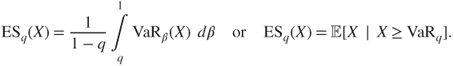
- If
 , the expected shortfall (ES) at confidence level
  is defined as
We will simplify the notation of those risk measures writing ![]() or
or ![]() when no confusion is possible.
when no confusion is possible.
Note that, in the case of an ![]() -Pareto distribution, analytical expressions of those two risk measures can be deduced from (11.2), namely,
-Pareto distribution, analytical expressions of those two risk measures can be deduced from (11.2), namely,
Recall also that the shape parameter ![]() totally determines the ratio
totally determines the ratio ![]() when we go far enough out into the tail:
when we go far enough out into the tail:
Note that this result holds also for the GPD with shape parameter ![]() .
.
When looking at aggregated risks ![]() , it is well known that the risk measure ES is coherent (see (Artzner et al., 1999)). In particular it is subadditive, that is,
, it is well known that the risk measure ES is coherent (see (Artzner et al., 1999)). In particular it is subadditive, that is,

whereas VaR is not a coherent measure, because it is not subadditive. Indeed many examples can be given where VaR is superadditive, that is,

see, e.g., Embrechts et al., (2009), Daníelsson et al., (2005).
In the case of ![]() -Pareto i.i.d. r.v.'s, the risk measure VaR is asymptotically superadditive (subadditive, respectively) if
-Pareto i.i.d. r.v.'s, the risk measure VaR is asymptotically superadditive (subadditive, respectively) if ![]() (
(![]() , respectively).
, respectively).
Recently, numerical and analytical techniques have been developed in order to evaluate the risk measures VaR and ES under different dependence assumptions regarding the loss r.v.'s. It certainly helps for a better understanding of the aggregation and diversification properties of risk measures, in particular of noncoherent ones such as VaR. We will not review these techniques and results in this report, but refer to Embrechts et al. (2013) for an overview and references therein. Let us add to those references some recent work by Mikosch and Wintenberger (2013) on large deviations under dependence which allows an evaluation of VaR. Nevertheless, it is worth mentioning a new numerical algorithm that has been introduced by Embrechts et al., (2013), which allows for the computation of reliable lower and upper bounds for the VaR of high-dimensional (inhomogeneous) portfolios, whatever the dependence structure is.
11.4.2 Possible Approximations of VaR
As an example, we treat the case of one of the two main risk measures and choose the VaR, since it is the main one used for solvency requirement. We would proceed in the same way for the expected shortfall.
It is straightforward to deduce, from the various limit theorems, the approximations ![]() of the VaR of order
of the VaR of order ![]() of the aggregated risks,
of the aggregated risks, ![]() , that is, the quantile of order
, that is, the quantile of order ![]() of the sum
of the sum ![]() defined by
defined by ![]() . The index
. The index ![]() indicates the chosen method, namely, (i) for the GCLT approach, (ii) for the CLT one, (iii) for the max one, (iv) for the Zaliapin et al.'s method, (v) for Normex, and (vi) for the weighted normal limit. We obtain the following:
indicates the chosen method, namely, (i) for the GCLT approach, (ii) for the CLT one, (iii) for the max one, (iv) for the Zaliapin et al.'s method, (v) for Normex, and (vi) for the weighted normal limit. We obtain the following:


11.4.3 Numerical Study: Comparison of the Methods
Since there is no explicit analytical formula for the true quantiles of ![]() , we will complete the analytical comparison of the distributions of
, we will complete the analytical comparison of the distributions of ![]() and
and ![]() given in Section 11.3.2.2, providing here a numerical comparison between the quantile of
given in Section 11.3.2.2, providing here a numerical comparison between the quantile of ![]() and the quantiles obtained by the various methods seen so far.
and the quantiles obtained by the various methods seen so far.
Nevertheless, in the case ![]() , we can compare analytically the VaR obtained when doing a rough normal approximation directly on
, we can compare analytically the VaR obtained when doing a rough normal approximation directly on ![]() , namely,
, namely, ![]() , with the one obtained via the shifted normal method, namely,
, with the one obtained via the shifted normal method, namely, ![]() . So, we obtain the correcting term to the CLT as
. So, we obtain the correcting term to the CLT as

11.4.3.1 Presentation of the study
We simulate ![]() with parent r.v.
with parent r.v. ![]()
![]() -Pareto distributed, with different sample sizes, varying from
-Pareto distributed, with different sample sizes, varying from ![]() (corresponding to aggregating weekly returns to obtain yearly returns) through
(corresponding to aggregating weekly returns to obtain yearly returns) through ![]() (corresponding to aggregating daily returns to obtain yearly returns) to
(corresponding to aggregating daily returns to obtain yearly returns) to ![]() representing a large size portfolio.
representing a large size portfolio.
We consider different shape parameters, namely, ![]() , respectively. Recall that simulated Pareto r.v.'s
, respectively. Recall that simulated Pareto r.v.'s ![]() 's (
's (![]() can be obtained simulating a uniform r.v.
can be obtained simulating a uniform r.v. ![]() on
on ![]() and then applying the transformation
and then applying the transformation ![]() .
.
For each ![]() and each
and each ![]() , we aggregate the realizations
, we aggregate the realizations ![]() 's (
's (![]() ). We repeat the operation
). We repeat the operation ![]() times, thus obtaining
times, thus obtaining ![]() realizations of the Pareto sum
realizations of the Pareto sum ![]() , from which we can estimate its quantiles.
, from which we can estimate its quantiles.
Let ![]() denote the empirical quantile of order
denote the empirical quantile of order ![]() of the Pareto sum
of the Pareto sum ![]() (associated with the empirical cdf
(associated with the empirical cdf ![]() and pdf
and pdf ![]() ) defined by
) defined by
Recall, for completeness, that the empirical quantile of ![]() converges to the true quantile as
converges to the true quantile as ![]() and has an asymptotic normal behavior, from which we deduce the following confidence interval at probability a for the true quantile:
and has an asymptotic normal behavior, from which we deduce the following confidence interval at probability a for the true quantile: ![]() , where
, where ![]() can be empirically estimated for such a large
can be empirically estimated for such a large ![]() . We do not compute them numerically:
. We do not compute them numerically: ![]() being very large, bounds are close.
being very large, bounds are close.
We compute the values of the quantiles of order ![]() ,
, ![]() (
(![]() indicating the chosen method), obtained by the main methods, the GCLT method, the Max one, Normex, and the weighted normal method, respectively. We do it for various values of
indicating the chosen method), obtained by the main methods, the GCLT method, the Max one, Normex, and the weighted normal method, respectively. We do it for various values of ![]() and
and ![]() . We compare them with the (empirical) quantile
. We compare them with the (empirical) quantile ![]() obtained via Pareto simulations (estimating the true quantile). For that, we introduce the approximative relative error:
obtained via Pareto simulations (estimating the true quantile). For that, we introduce the approximative relative error:

We consider three possible order ![]() :
: ![]() ,
, ![]() (threshold for Basel II) and
(threshold for Basel II) and ![]() (threshold for Solvency 2).
(threshold for Solvency 2).
We use the software R to perform this numerical study, with different available packages. Let us particularly mention the use of the procedure Vegas in the package R2Cuba for the computation of the double integrals. This procedure turns out not to be always very stable for the most extreme quantiles, mainly for low values of ![]() . In practice, for the computation of integrals, we would advise to test various procedures in R2Cuba (Suave, Divonne, and Cuhre, besides Vegas) or to look for other packages. Another possibility would be implementing the algorithm using altogether a different software, as, for example, Python.
. In practice, for the computation of integrals, we would advise to test various procedures in R2Cuba (Suave, Divonne, and Cuhre, besides Vegas) or to look for other packages. Another possibility would be implementing the algorithm using altogether a different software, as, for example, Python.
11.4.3.2 Estimation of the VaR with the various methods
All codes and results are obtained for various ![]() and
and ![]() are given in Kratz (2013) (available upon request) and will draw conclusions based on all the results.
are given in Kratz (2013) (available upon request) and will draw conclusions based on all the results.
We start with a first example when ![]() to illustrate our main focus, when looking at data under the presence of moderate heavy tail. We present here the case
to illustrate our main focus, when looking at data under the presence of moderate heavy tail. We present here the case ![]() in Table 11.4.
in Table 11.4.
Table 11.4 Approximations of extreme quantiles (95%; 99%; 99.5%) by various methods (CLT, Max, Normex, weighted normal) and associated approximative relative error to the empirical quantile ![]() , for n = 52, 100, 250, 500 respectively, and
, for n = 52, 100, 250, 500 respectively, and ![]()
| 95% | 103.23 | 104.35 | 102.60 | 103.17 | 109.25 |
| 1.08 | 5.83 | ||||
| 99% | 119.08 | 111.67 | 117.25 | 119.11 | 118.57 |
| 0.03 | |||||
| 99.5% | 128.66 | 114.35 | 127.07 | 131.5 | 121.98 |
| 2.21 | |||||
| 95% | 189.98 | 191.19 | 187.37 | 189.84 | 197.25 |
| 0.63 | 3.83 | ||||
| 99% | 210.54 | 201.35 | 206.40 | 209.98 | 209.74 |
| 99.5% | 222.73 | 205.06 | 219.14 | 223.77 | 214.31 |
| 0.47 | |||||
| 95% | 454.76 | 455.44 | 446.53 | 453.92 | 464.28 |
| 0.17 | 2.09 | ||||
| 99% | 484.48 | 471.5 | 473.99 | 483.27 | 483.83 |
| 99.5% | 501.02 | 477.38 | 492.38 | 501.31 | 490.98 |
| 0.06 | |||||
| 95% | 888.00 | 888.16 | 872.74 | 886.07 | 900.26 |
| 0.02 | 1.38 | ||||
| 99% | 928.80 | 910.88 | 908.97 | 925.19 | 927.80 |
| 99.5% | 950.90 | 919.19 | 933.23 | 948.31 | 937.89 |
Let us also illustrate in table 11.5 the heavy tail case, choosing, for instance, ![]() , which means that
, which means that ![]() . Take, for example,
. Take, for example, ![]() respectively, to illustrate the fit of Normex even for small samples. Note that the weighted normal does not apply here since
respectively, to illustrate the fit of Normex even for small samples. Note that the weighted normal does not apply here since ![]() .
.
Table 11.5 Approximations of extreme quantiles (95%; 99%; 99.5%) by various methods (GCLT, Max, Normex) and associated approximative relative error to the empirical quantile ![]() , for
, for ![]() , respectively, and for
, respectively, and for ![]()
| 95% | 246.21 | 280.02 | 256.92 | 245.86 |
| 13.73 | 4.35 | |||
| 99% | 450.74 | 481.30 | 455.15 | 453.92 |
| 6.78 | 0.97 | 0.71 | ||
| 99.5% | 629.67 | 657.91 | 631.66 | 645.60 |
| 4.48 | 0.31 | 2.53 | ||
| 95% | 442.41 | 491.79 | 456.06 | 443.08 |
| 11.16 | 3.09 | 0.15 | ||
| 99% | 757.82 | 803.05 | 762.61 | 761.66 |
| 5.97 | 0.63 | 0.51 | ||
| 99.5% | 1031.56 | 1076.18 | 1035.58 | 1032.15 |
| 4.33 | 0.39 | 0.06 |
11.4.3.3 Discussion of the results
- Those numerical results are subject to numerical errors due to the finite sample of simulation of the theoretical value, as well as the choice of random generators, but the most important reason for numerical error of our methods resides in the convergence of the integration methods. Thus, one should read the results, even if reported with many significant digits, to a confidence we estimate to be around 0.1% (also for the empirical quantiles).
- The Max method overestimates for
 and underestimates for
  ; it improves a bit for higher quantiles and
  . It is a method that practitioners should think about when wanting to have a first idea on the range of the VaR, because it is very simple to use and costless in terms of computations. Then they should turn to Normex for an accurate estimation.
 - The GCLT method (
 ) overestimates the quantiles but improves with higher quantiles and when
  increases.
 - Concerning the CLT method (
 ), we find out that:
- The higher the quantile, the higher the underestimation; it improves slightly when
 increases, as expected.
 - The smaller
 , the larger the underestimation.
 - The estimation improves for smaller-order
 of the quantile and large
  , as expected, since, with smaller order, we are less in the upper tail.
 - The VaR estimated with the normal approximation is almost always lower than the VaR estimated via Normex or the weighted normal method. The lower
 and
and  , the higher the difference with Normex.
 - The difference between the VaR estimated by the CLT and the one estimated with Normex appears large for relatively small
 , with a relative error going up to 13%, and decreases when
  becomes larger.
- The higher the quantile, the higher the underestimation; it improves slightly when
- With the Weighted Normal method (
 ), it appears that:
- The method overestimates the 95% quantile but is quite good for the 99% one. In general, the estimation of the two upper quantiles improve considerably when compared with the ones obtained via a straightforward application of the CLT.
- The estimation of the quantiles improve with increasing n and increasing
 .
. - The results are generally not as sharp as the ones obtained via Normex, but better than the ones obtained with the max method, whenever
 .
.
- Concerning Normex, we find out that:
- The accuracy of the results appears more or less independent of the sample size
 , which is the major advantage of our method when dealing with the issue of aggregation.
 - For
 , it always gives sharp results (error less than 0.5% and often extremely close); for most of them, the estimation is indiscernible from the empirical quantile, obviously better than the ones obtained with the other methods.
 - For
 , the results for the most extreme quantile are slightly less satisfactory than expected. We attribute this to a numerical instability in the integration procedure used in R. Indeed, for very large quantiles (
 %), the convergence of the integral seems a bit more unstable (due to the use of the package Vegas in R), which may explain why the accuracy decreases a bit and may sometimes be less than with the Max method. This issue should be settled using other R-package or software.
- The accuracy of the results appears more or less independent of the sample size
- We have concentrated our study on the VaR risk measure because it is the one used in solvency regulations both for banks and insurances. However, the expected shortfall, which is the only coherent measure in presence of fat tails, would be more appropriate for measuring the risk of the companies. The difference between the risk measure estimated by the CLT and the one estimated with Normex would certainly be much larger than what we obtain with the VaR when the risk is measured with the expected shortfall, pleading for using this measure in presence of fat tails.
11.4.3.4 Normex in practice
From the results we obtained, Normex appears as the best method among the ones we studied, applicable for any ![]() and
and ![]() . This comparison was done on simulated data. A next step will be to apply it on real data.
. This comparison was done on simulated data. A next step will be to apply it on real data.
Let us sketch up a step-by-step procedure on how Normex might be used and interpreted in practice on real data when considering aggregated heavy-tailed risks.
We dispose of a sample ![]() , with unknown heavy-tailed cdf having positive tail index
, with unknown heavy-tailed cdf having positive tail index ![]() . We order the sample as
. We order the sample as ![]() and consider the aggregated risks
and consider the aggregated risks ![]() that can be rewritten as
that can be rewritten as ![]() .
.
- Preliminary step: Estimation of
 , with standard EVT methods (e.g., Hill estimator (Hill, 1975)),
  -estimator (Kratz and Resnick, 1996); (Beirlant et al., 1996)), etc.); let
  be denoted as an estimate of
  .
. - Define
 with
with  (see (11.13)); the
  largest order statistics share the property of having a
  th infinite moment, contrary to the
  first ones. Note that
  is independent of the aggregation size.
 - The
 first order statistics and the
  last ones being, conditionally on
  , independent, we apply the CLT to the sum of the
  first order statistics conditionally on
  and compute the distribution of the sum of the last
  ones conditionally on
  assuming a Pareto distribution for the r.v.'s because of (11.3).
 - We can then approximate the cdf of
 by
by  defined in Theorem 11.2, which provides a sharp approximation, easily computable whatever the size of the sample is.
 - We deduce any quantile
 of order
  of
of  as
as  , which allows an accurate evaluation of risk measures of aggregated heavy-tailed risks.
11.5 Conclusion
The main motivation of this study was to propose a sharp approximation of the entire distribution of aggregate risks when working on financial or insurance data under the presence of fat tails. It corresponds to one of the daily duties of actuaries when modeling investment or insurance portfolios. In particular the aim is to obtain the most accurate evaluations of risk measures. After reviewing the existing methods, we built two new methods, Normex and the weighted normal method. Normex is a method mixing a CLT and the exact distribution for a small number (defined according to the range of ![]() and the choice of the number of existing moments of order
and the choice of the number of existing moments of order ![]() ) of the largest order statistics. The second approach is based on a weighted normal limit, with a shifted mean and a weighted variance, both expressed in terms of the tail distribution.
) of the largest order statistics. The second approach is based on a weighted normal limit, with a shifted mean and a weighted variance, both expressed in terms of the tail distribution.
In this study, Normex has been proved, theoretically as well as numerically, to deliver a sharp approximation of the true distribution, for any sample size ![]() and for any positive tail index
and for any positive tail index ![]() , and is generally better than existing methods. The weighted normal method consists of trimming the total sum by taking away a large number of extremes and approximating the trimmed sum with a normal distribution and then shifting it by the (almost sure) limit of the average of the extremes and correcting the variance with a weight depending on the shape of the tail. It is a simple and reasonable tool, which allows to express explicitly the tail contribution to be added to the VaR when applying the CLT to the entire sample. It has been developed empirically in this work and still requires further analytical study. It constitutes a simple and exploratory tool to remediate the underestimation of extreme quantiles over 99% .
, and is generally better than existing methods. The weighted normal method consists of trimming the total sum by taking away a large number of extremes and approximating the trimmed sum with a normal distribution and then shifting it by the (almost sure) limit of the average of the extremes and correcting the variance with a weight depending on the shape of the tail. It is a simple and reasonable tool, which allows to express explicitly the tail contribution to be added to the VaR when applying the CLT to the entire sample. It has been developed empirically in this work and still requires further analytical study. It constitutes a simple and exploratory tool to remediate the underestimation of extreme quantiles over 99% .
An advantage of both methods, Normex and the weighted normal, is their generality. Indeed, trimming the total sum by taking away extremes having infinite moments (of order ![]() ) is always possible and allows to better approximate the distribution of the trimmed sum with a normal one (via the CLT). Moreover, fitting a normal distribution for the mean behavior can apply, not only for the Pareto distribution but for any underlying distribution, without having to know about it, whereas for the extreme behavior, we pointed out that a Pareto type is standard in this context.
) is always possible and allows to better approximate the distribution of the trimmed sum with a normal one (via the CLT). Moreover, fitting a normal distribution for the mean behavior can apply, not only for the Pareto distribution but for any underlying distribution, without having to know about it, whereas for the extreme behavior, we pointed out that a Pareto type is standard in this context.
Normex could also be used from another point of view. We could apply it for a type of inverse problem to find out a range for the tail index ![]() when fitting this explicit mixed distribution to the empirical one. Note that this topic of tail index estimation has been studied extensively in the literature on the statistics of extremes (see, e.g., (Beirlant et al., 2004); (Reiss and Thomas, 2007), and references therein). Approaches to this estimation may be classified into two classes, supervised procedures in which the threshold to estimate the tail is chosen according to the problem (as, e.g., for seminal references, the weighted moments (Hosking and Wallis, 1987)), the MEP (Davison and Smith, 1990); (Hill, 1975),
when fitting this explicit mixed distribution to the empirical one. Note that this topic of tail index estimation has been studied extensively in the literature on the statistics of extremes (see, e.g., (Beirlant et al., 2004); (Reiss and Thomas, 2007), and references therein). Approaches to this estimation may be classified into two classes, supervised procedures in which the threshold to estimate the tail is chosen according to the problem (as, e.g., for seminal references, the weighted moments (Hosking and Wallis, 1987)), the MEP (Davison and Smith, 1990); (Hill, 1975), ![]() (Kratz and Resnick, 1996); (Beirlant et al., 1996)) methods, and unsupervised ones, where the threshold is algorithmically determined (as, e.g., in (Bengio and Carreau, 2009) and references therein, (Debbabi and Kratz, 2014)). Normex would then be classified as a new unsupervised approach, since the
(Kratz and Resnick, 1996); (Beirlant et al., 1996)) methods, and unsupervised ones, where the threshold is algorithmically determined (as, e.g., in (Bengio and Carreau, 2009) and references therein, (Debbabi and Kratz, 2014)). Normex would then be classified as a new unsupervised approach, since the ![]() is chosen algorithmically for a range of
is chosen algorithmically for a range of ![]() .
.
Other perspectives concern the application of this study to real data, its extension to the dependent case, using CLT under weak dependence and some recent results on stable limits for sums of dependent infinite variance r.v. from Bartkiewicz et al. (2012) and large deviation principles from (Mikosch and Wintenberger, 2013).
Finally this study may constitute a first step in understanding the behavior of VaR under aggregation and be helpful in analyzing the scaling behavior of VaR under aggregation, next important problem that we want to tackle.
References
- Acerbi, C., Tasche, D. On the coherence of expected shortfall. Journal of Banking & Finance 2002;26:1487–1503.
- Artzner, P., Delbaen, F., Eber, J.-M., Heath, D. Coherent measures of risks. Mathematical Finance 1999;9:203–228.
- Bartkiewicz, K., Jakubowski, A., Mikosch, T., Wintenberger, O. Stable limits for sums of dependent infinite variance random variables. Probab Theory Relat Fields 2012;150:337–372.
- Basel Committee on Banking Supervision. Developments in modelling risk aggregation. Basel: Bank for International Settlements; 2010.
- Beirlant, J., Goegebeur, Y., Segers, J., Teugels, J. Statistics of Extremes: Theory and Applications. New York: John Wiley & Sons, Inc.; 2004.
- Beirlant, J., Vynckier, P., Teugels, J. Tail index estimation, Pareto quantile plots, and regression diagnostics. J Am Stat Assoc 1996;91:1659–1667.
- Bellini, F., Klar, B., Müller, A., Rosazza Gianin, E. Generalized quantiles as risk measures; 2013. Preprint http://ssrn.com/abstract=2225751. Accessed 2016 May 2.
- Bengio, Y., Carreau, J. A hybrid Pareto model for asymmetric fat-tailed data: the univariate case. Extremes 2009;1:53–76.
- Cai, G.-H. The Berry-Esséen bound for identically distributed random variables by Stein method. Appl Math J Chin Univ 2012;27:455–461.
- Chen, L.H., Shao, Q.-M. Normal approximation under local dependence. Ann Probab 2004;32(3):1985–2028.
- Csörgö, S., Horváth, L., Mason, D. What portion of the sample makes a partial sum asymptotically stable or normal? Probab Theory Relat Fields 1986;72:1–16.
- Dacorogna, M.M., Gençay, R., Müller, U., Olsen, R., Pictet, O. An Introduction to High-Frequency Finance. New York: Academic Press; 2001.
- Dacorogna, M.M., Müller, U.A., Pictet, O.V., de Vries, C.G. The distribution of extremal foreign exchange rate returns in extremely large data sets. Extremes 2001;4(2):105–127.
- Daníelsson, J., Jorgensen, B., Samorodnitsky, G., Sarma, M., de Vries, C. Subadditivity re-examined: the case for Value-at-Risk. FMG Discussion Papers, London School of Economics; 2005.
- David, H.A., Nadaraja, H.N. Order Statistics. 3rd ed. New York: John Wiley & Sons, Inc.; 2003.
- Davison, A., Smith, R. Models for exceedances over high thresholds. J R Stat Soc Ser B 1990;52(3):393–442.
- Debbabi, N., Kratz, M. A new unsupervised threshold determination for hybrid models. IEEE-ICASSP; 2014.
- Embrechts, P., Klüppelberg, C., Mikosch, T. Modelling Extremal Events for Insurance and Finance. Berlin: Springer-Verlag; 1997.
- Embrechts, P., Lambrigger, D., Wüthrich, M. Multivariate extremes and the aggregation of dependent risks: examples and counter-examples. Extremes 2009;12:107–127.
- Embrechts, P., Puccetti, G., Rüschendorf, L. Model uncertainty and VaR aggregation. Journal of Banking & Finance 2013;37(8):2750–2764.
- Emmer, S., Kratz, M., Tasche, D. What is the best risk measure in practice? A comparison of standard risk measures. J Risk 2015;18:31-60.
- Esseen, C.-G. On the Liapunoff limit of error in the theory of probability. Ark Mat Astron Fysik 1942;A28:1–19. ISSN: 0365-4133.
- Feller, W. An Introduction to Probability Theory and its Applications. Volume II. New York: Wiley; 1966.
- Fisher, R.A., Tippett, L.H.C. Limiting forms of the frequency distribution of the largest or smallest member of a sample. Proc Camb Philos Soc 1928;24:180–190.
- Furrer, H. Uber die Konvergenz zentrierter und normierter Summen von Zufallsvariablen und ihre Auswirkungen auf die Risikomessung; 2012. ETH preprint.
- Galambos, J. The Asymptotic Theory of Extreme Order Statistics. New York: John Wiley & Sons, Inc.; 1978.
- Gneiting, T. Making and evaluating point forecasts. J Am Stat Assoc 2012;106(494):746–762.
- Hahn, M.G., Mason, D.M., Weiner, D.C. Sums, Trimmed Sums and Extremes. Progress in Probability. Volume 23. Cambridge (MA): Birkhäuser Boston; 1991.
- Hall, P. On the influence of extremes on the rate of convergence in the central limit theorem. Ann Probab 1984;12:154–172.
- Hill, B.M. A simple approach to inference about the tail of a distribution. Ann Stat 1975;3:1163–1174.
- Hosking, J., Wallis, J. Parameter and quantile estimation for the Generalized Pareto distribution. Technometrics 1987;29(3):339–349.
- Hosking, J.R.M., Wallis, J.R., Wood, E.F. Estimation of the generalized extreme-value distribution by the method of probability-weighted moments. Technometrics 1985;27:251–261. [321–323].
- Huston, J., McCulloch, M. Measuring tail thickness to estimate the stable index
 : a critique. J. of Business & Economic Statistics 1997;15:74–81.
 - Jansen, D.W., De Vries, C.G. On the frequency of large stock returns: putting booms and busts into perspectives. Review of Economics and Statistics 1991;73:18–24.
- Jenkinson, A.F. The frequency distribution of the annual maximum (or minimum) values of meteorological elements. Q J R Meteorol Soc 1955;81:58–171.
- Korolev, V.Y., Shevtsova, I.G. On the upper bound for the absolute constant in the Berry-Esseen inequality. J Theory Probab Appl 2010;54(4):638–658.
- Kratz, M. There is a VaR beyond usual approximations. Towards a toolkit to compute risk measures of aggregated heavy tailed risks. FINMA report; 2013.
- Kratz, M. Normex, a new method for evaluating the distribution of aggregated heavy tailed risks. Application to risk measures. Extremes 2014;17(4) (Special issue: Extremes and Finance. Guest Ed. P. Embrechts). 661–691.
- Kratz, M., Resnick, S. The QQ-estimator and heavy tails. Stoch Models 1996;12:699–724.
- Leadbetter, R., Lindgren, G., Rootzén, H. Extremes and Related Properties of Random Sequences and Processes. New York: Springer-Verlag; 1983.
- Longin, F. The asymptotic distribution of extreme stock market returns. J Bus 1996;63:383–408.
- Mikosch, T., Wintenberger, O. Precise large deviations for dependent regularly varying sequences. Probab Theory Relat Fields 2013;156:851–887.
- Mori, T. On the limit distribution of lightly trimmed sums. Math Proc Camb Philos Soc 1984;96:507–516.
- Müller, U.A., Dacorogna, M.M., Pictet, O.V. Heavy tails in high-frequency financial data. In: Taqqu, M., editor. Published in the book A Practical Guide to Heavy Tails: Statistical Techniques for Analysing Heavy Tailed Distributions. Boston (MA): Birkhauser; 1998.
- Nolan, J. 2012. Available at http://academic2.american.edu/jpnolan/stable/stable.html. Accessed 2016 May 2.
- Petrov, V.V. A local theorem for densities of sums of independent random variables. J Theory Probab Appl 1956;1(3):316–322.
- Petrov, V.V. Limit Theorem of Probability Theory: Sequences of Independent Random Variables. Oxford: Oxford Sciences Publications; 1995.
- Pickands, J. Statistical inference using extreme order statistics. Ann Stat 1975;3:119–131.
- Pictet, O., Dacorogna, M., Müller, U.A. Hill, Bootstrap and Jackknife Estimators for heavy tails, In: Taqqu, M., editor. Practical Guide for Heavy Tails Distributions. Boston (MA): Birkhäuser; 1998.
- Pinelis, I. On the nonuniform Berry-Esséen bound; 2013. arxiv.org/pdf/1301.2828.
- Ramsay, C.M. The distribution of sums of certain i.i.d. Pareto variates. Commun Stat Theory Methods 2006;35(3):395–405.
- Reiss, R.-D., Thomas, M. Statistical Analysis of Extreme Values: With Applications to Insurance, Finance, Hydrology and Other Fields. 3rd ed. Birkhäuser Basel; 2007.
- Resnick, S. Extreme Values, Regular Variation, and Point Processes. 1st ed. New York: Springer-Verlag; 1987, 2008.
- Resnick, S. Heavy-Tail Phenomena: Probabilistic and Statistical Modeling. New York: Springer-Verlag; 2006.
- Samorodnitsky, G., Taqqu, M.S. Stable non-Gaussian Random Processes: Stochastic Models with Infinite Variance. New York: Chapman & Hall; 1994.
- Shevtsova, I.G. About the rate of convergence in the local limit theorem for densities under various moment conditions. Statistical Methods of Estimation and Hypotheses Testing Volume 20, Perm, Russia; 2007. p 1-26(in Russian).
- Shevtsova, I.G. On the absolute constants in the Berry-Esséen inequality and its structural and nonuniform improvements. Informatics and its Applications 2013;7(1):124–125 (in Russian).
- Stein, C. A bound for the error in the normal approximation to the distribution of a sum of dependent random variables. Proceedings of the 6th Berkeley Symposium on Mathematical Statistics and Probability, Volume 2; 1972. p 583–602.
- Stein, C. Approximate Computations of Expectations. Volume 7, Lecture Notes—Monograph Series. Hayward (CA): IMS; 1986.
- Taylor, S.J. Modelling Financial Time Series. Chichester: John Wiley & Sons; 1986.
- Tyurin, I.S. An improvement of upper estimates of the constants in the Lyapunov theorem. Russian Mathematical Surveys 2010;65(3):201–202.
- von Mises, R. La distribution de la plus grande de n valeurs. Revue Mathématique de l'Union Interbalkanique 1936;1:141–160.
- Zaliapin, I.V., Kagan, Y.Y., Schoenberg, F.P. Approximating the distribution of Pareto sums. Pure Appl Geophys 2005;162:1187–1228.
- Ziegel, J.F. Coherence and elicitability. Mathematical Finance 2014 (online 2014).