
Chapter 13
Comparing Tail Risk and Systemic Risk Profiles for Different Types of U.S. Financial Institutions
Stefan Straetmans and Thanh Thi Huyen Dinh
School of Business and Economics, Maastricht University, Maastricht, The Netherlands
JEL codes: G21, G28, G29, G12, C49.
13.1 Introduction
The Basel II framework identifies credit risk, market risk, and operational risk as the key risk factors for financial institutions. Prior to the Crisis, the dominant opinion used to be that by appropriately managing these risks, financial institutions can maximize the probability of their continued survival while delivering appropriate profit to the capital providers. However, this financial regulatory framework is essentially micro-prudential in nature in the sense that it is designed to limit each institution's risk individually. However, Basel II typically did not take into account that distressed systemically important companies can destabilize the whole financial system as well as causing negative effects on real economic activity. The recent financial crisis created a conscience that there is an urgent need to complement Basel II with regulations that also take into account these macro-prudential concerns, that is, the need to monitor the so-called systemic risk. Thus, in order to preserve monetary and financial stability, central banks, as well as regulatory and supervisory authorities (often one and the same entity), ideally should have a regulatory and supervisory framework that both exhibits a micro-prudential layer as well as a set of tools to monitor the systemic importance of individual financial institutions in order to get a feel of the potential for the overall financial sector instability. This is a particularly challenging task in large and complex economies with highly developed financial systems. In the United States, for example, tremendous consolidation as well as the removal of regulatory barriers to universal banking has made the financial system's interconnectedness extremely complex, giving rise to the popular reference to the so-called large and complex banking organizations (or LCBOs) as institutions that are “too complex to fail.”
A significant body of theoretical and empirical literature on bank contagion and systemic risk developed throughout the years, but the amount of scientific contributions in this area has nearly exploded since the occurrence of the most recent systemic banking crisis. A majority of the empirical banking stability literature has proposed “market-based” indicators of systemic risk. That is because factors that are supposed to drive systemic instability, such as, for example, the financial system's interbank interconnectedness, the location of banks within the system's “network,” or the correlations between loan or trading (investment) portfolios are often difficult to quantify. Banks' interconnectedness may be “direct,” that is, related to money markets, the payment system, or derivatives markets and the resulting counterparty risk, see, for example, Allen and Gale (2000). However, it may also be of an “indirect” nature and induced by the overlap in banks' asset portfolios (Iori et al., 2006; De Vries, 2005; Zhou, 2010). Event studies are one of the oldest tools employed to measuring bank linkages by investigating the impacts of specific bank distress or bank failures on other banks' stock prices, see, for example, Swary (1986), Wall and Peterson (1990), or Slovin et al. (1999). Other studies ran regressions of abnormal bank stock returns on proxies for asset-side risk, for example, Smirlock and Kaufold (1987) or Kho et al. (2000). De Nicolo and Kwast (2002) explain increases in bank equity correlations over time by means of proxies for bank consolidation. Gropp and Moerman (2004) and Gropp and Vesala (2004) use (market-based) equity-derived distances to default to measure bank equity spillovers. More recent market-based measures of systemic risk include the Shapley value (Tarashev et al., 2010), conditional value at risk (VaR) (Adrian and Brunnermeier, 2011), marginal expected shortfall (MES) (Acharya et al., 2011), or SRISK (Brownlees and Engle, 2015).
All the studies mentioned above assumed that domino-type bank equity spillovers (often dubbed “bank contagion”) are at the heart of systemic risk. An alternative strand in the literature assumes that banking crises are triggered by aggregate (nondiversifiable) shocks that affect all banks simultaneously. The systemic risk indicator we are going to work with fits into this latter tradition. Gorton (1988) argued that business cycles have often been leading indicators of bank panics. The studies by Gonzalez-Hermosillo et al. (1997) (for Mexico), Demirgüc-Kunt and Detragiache (1998) (multi-country-evidence), and Hellwig (1994) fit in the same tradition. The latter author argued that the fragility of financial institutions to large macro shocks may partly be due to the noncontingent character of deposit contracts to the state of the macro economy.
The use of market-based indicators for systemic risk is not without controversy and potential problems. First, it allows systemic risk assessment only for listed banks. This may lead to a biased view on the true level of financial fragility. Second, bank stocks can be truly informative about current or future systemic risk (i.e., market-based indicators as “early warning indicator”) only if bank stocks reflect all relevant and available information about the risks that characterize a given financial institution, that is, if bank stocks are efficiently priced. In efficient stock markets, large drops in the market value of bank equity should occur only (i) when there is institution-specific news about that bank; (ii) when there is institution-specific news about related banks; (iii) in the presence of adverse aggregate shocks that impact all banks simultaneously. The evolution of bank stocks prior to 2007 rather suggests that the markets did not foresee the banking crisis. We nevertheless believe that the extreme spikes in bank stocks and their co-movements exhibit at least some informational content about systemic risk and stability.
This chapter builds on the statistical extreme value theory (EVT) approach followed by, for example, Hartmann et al. (2006) and Straetmans and Chaudhry (2015). More specifically, we use extreme downside risk measures that assume Pareto-type tail decline. To identify bank systemic risk, we employ the so-called tail-β indicator of “extreme systematic” risk as a tail equivalent of the traditional regression-based CAPM-β, introduced in Straetmans et al. (2008). Tail-β is defined as the probability of a collapse in the market value of a bank's equity capital conditional on a large adverse aggregate shock (typically an extreme negative return on a market portfolio like a banking index, overall stock market index, credit spread, etc.). Tail-β is obviously market-based because it uses stock prices of individual bank equity as well as market-based information about aggregate shocks (i.e., market indices for the banking sector).
Notice that the concept of MES and the conditional value at risk (CoVaR) resemble tail-β because these indicators are also probabilistic in nature: MES is the expected loss on individual bank equity capital conditional on large market portfolio losses; CoVaR is the VaR of the financial system conditional on institutions being under distress and is implicitly defined using a conditional co-crash probability. Also, and in contrast to previous correlation-based approaches toward modeling market linkages and spillovers, MES, CoVaR, and tail-β identify nonlinear dependencies (if present) in the data. The crucial difference between our approach and competing approaches such as MES or CoVaR lies in the way the indicators are estimated: whereas we explicitly focus on the extreme tails of bank equity capital and the tail dependence structure between bank stock returns, parallel studies identifying MES or CoVaR typically use estimation techniques like quantile regressions that do not go as far in the tail. They typically assume that non-extreme outcomes are representative for what happens in the tail area but we believe this may be an overly restrictive assumption. Statistical EVT deals with events that are severe enough for regulators and supervisors caring about financial stability, which cannot be claimed about events that happen 5% of 1% of the time.
By applying techniques of univariate and multivariate EVT to the tails of bank equity returns, we make four contributions to the existing literature. First, we perform a “cross-industry” comparison of tail risk and systemic importance, that is, do traditional banks exhibit more or less tail risk and systemic risk as compared to, for example, investment banks or insurance companies? Indeed, besides deposit banks, insurance companies (including large reinsurers) and B&Ds (investment banks) played a crucial role in the narrative of the 2007–2009 banking and financial crisis. It is to be expected that these different segments of the financial industry also exhibit different risk profiles and risk-taking behavior. Previous empirical systemic risk studies were often limited to measuring tail risk and systemic risk of banks in the narrow sense of the word. Second, we assess the forward-looking characteristics of these risk measures by looking at the stability of tail risk and systemic risk rankings over time. We therefore calculate rank correlations between pre-crisis and crisis ranks. Third, we reinvestigate the corroboration that a financial institution's size is a prime factor fueling systemic risk. We also look into the relation between tail risk and institutional size. Finally, we want to assess whether the tail risk and systemic risk of the same institutions are positively or negatively related to each other. Suppose that both micro-prudential (tail) risk and macro-prudential (systemic) risk exhibit common drivers; the relation between the common factors and the two risk types and their common drivers will also determine whether tail risk and systemic risk are positively or negatively related. For example, if size is the single most important variable and bigger banks exhibit less tail risk (diversification effect) but more systemic risk (too big to fail effect), then it follows that tail risk and systemic risk should be negatively related to each other across financial institutions. Whether tail risk and systemic risk are positively or negatively correlated is assessed by means of cross-sectional rank correlations between tail risk and systemic risk for the pre-crisis and the crisis subsample separately.
Turning to the data, our panel contains roughly the same banks as in Acharya et al. (2011) and Brownlees and Engle (2015), that is, the top 102 U.S. financial firms with a market capitalization greater than 7 billion USD as of the end of June 2007 (just before the start of the subprime mortgage crisis). SIC codes are used to divide financial institutions into four buckets: deposit banks (e.g., JP Morgan, Bank of America, Citigroup), insurance companies (e.g., AIG, Berkshire Hathaway, Countrywide), B&Ds (e.g., Goldman Sachs, Morgan Stanley), and a residual category (“others”) consisting of nondepository institutions or real estate agencies. Our dataset includes only 92 firms instead of the 102 as in the original panel due to mergers or bankruptcies. Stock prices and relevant balance sheet data to proxy institutional size are downloaded over the sample period January 1, 1990 to September 1, 2011.
Anticipating our results, we find that different groups of financial institutions exhibit different levels of tail risk and systemic risk. The heterogeneity in tail risks and systemic contributions across different types of financial institutions suggests that a tailor-made regulatory and supervisory approach may be advisable. The most salient outcome of our cross-industry risk comparison, however, seems to be that the insurance industry exhibits the highest tail risk but that deposit banks are characterized by the highest degree of extreme systematic risk. The latter outcome is surprising given the role investment banks (and more specifically the trading divisions) seem to have played in the narrative of the financial crisis. What is less surprising is that both tail risk and systemic risk dramatically increased during the financial crisis. However, this does not mean that EVT-based indicators of tail risk and systemic risk are of no value when making any judgment about the propensity toward future systemic crises: we actually observe that the ranking of institutions did not change dramatically when considering pre-crisis and crisis tail-βs: the riskiest institutions in terms of tail risk and systemic risk before the crisis stay the riskiest ones over the crisis sample. The ranking stability is nevertheless quite fluctuating across different types of financial institutions. Last but not least, financial institutions' size does not have much to say about financial institutions' tail risk; but size does seem to matter for their systemic risk. However, the size–systemic risk relationship is not very robust and varies with the considered size proxies, subsamples, and types of financial institutions.
The remainder of this chapter is organized as follows. Section 13.2 introduces indicators of downside risk and systemic risk based on statistical extreme value analysis. Section 13.3 provides estimation procedures for both measures. Section 13.4 summarizes the empirical results. Section 13.5 concludes.
13.2 Tail Risk and Systemic Risk Indicators
We first introduce alternative downside risk measures for financial institutions (Section 13.2.1). Next, we discuss a systemic risk indicator that reflects individual banks' sensitivity to systemwide, nondiversifiable shocks (tail-β) (Section 13.2.2).
13.2.1 Univariate Tail Risk Indicators
We define extreme downside risk (tail risk) measures for financial institutions by exploiting the empirical stylized fact that equity returns of financial institutions exhibit “heavy” tails. Mandelbrot (1963) was arguably the first to observe that sharp short-term fluctuations in financial markets (typically daily returns) are nonnormally distributed – and bank stocks do not constitute an exception. Let ![]() stand for the dividend-corrected stock price of a financial institution. Define
stand for the dividend-corrected stock price of a financial institution. Define ![]() as the loss variable we are interested in. For the sake of notational convenience, the left tail of equity returns (market losses on equity capital) is mapped into positive losses, which implies that all downside risk measures are expressed for the upper tail of a loss distribution. Loosely speaking, Mandelbrot's observation of the heavy-tail feature implies that the marginal tail probability for X as a function of the corresponding quantile can be approximately described by a power law
as the loss variable we are interested in. For the sake of notational convenience, the left tail of equity returns (market losses on equity capital) is mapped into positive losses, which implies that all downside risk measures are expressed for the upper tail of a loss distribution. Loosely speaking, Mandelbrot's observation of the heavy-tail feature implies that the marginal tail probability for X as a function of the corresponding quantile can be approximately described by a power law
for large x.
This contrasts with the (much faster) exponential tail decay of thin-tailed processes like the normal distribution. The so-called tail index α can be interpreted as the rate at which the tail decay takes place when making the quantile or crisis barrier x more extreme: a lower α implies a slower decay to zero and a higher probability mass for given values of x. The tail index also has an interesting statistical interpretation in terms of the higher moments of an empirical process: all distributional moment higher than α are unbounded and thus do not exist. In contrast, for the normal distribution, all statistical moments exist. Mandelbrot's empirical observation of heavy tails implies that the normal distribution is not a good choice if one wants to make probability assessment of extreme returns such as financial crises, bank failures, and so on. Why is the normality assumption still so common when applying statistical tools to social sciences? This can be partly explained by (i) its analytical tractability, and, more importantly, (ii) by the predominant focus on sample averages in social science, which implies that versions of the central limit theorem apply. However, if one is interested in assessing the likelihood of extreme events (financial crises, bank distress, etc.) away from the mean and the distributional center, other limit laws apply, such as the extremal types theorem, see Embrechts et al. (1997). The heavy-tailed model (13.1) is one possible outcome of this extremal types theorem.
Popular distributional models often used in the finance literature, such as the Student-t, the class of symmetric stable distributions, or the generalized autoregressive conditional heteroscedasticity (GARCH) model, all exhibit fat tails: they are all nested in the tail model (13.1) albeit with different pairs of tail parameters ![]() .
.
Clearly, the tail likelihood in (13.1) is defined for a given time horizon of the loss series X and values of the crisis barrier or VaR level ![]() . Alternatively, (13.1) can be inverted and solved for the tail quantile x as a function of p:
. Alternatively, (13.1) can be inverted and solved for the tail quantile x as a function of p:
Although VaR has become an extremely popular device for financial risk management and even a cornerstone of Basel II, financial economists also argue it is not a “coherent” risk measure; alternative risk measures have therefore been proposed, like, for example, the “expected shortfall” (i.e., the conditional expected loss on a firm's equity capital given a sharp decline in equity capital ![]() ). It can be easily shown that the expected shortfall is very closely related to the VaR:
). It can be easily shown that the expected shortfall is very closely related to the VaR:
Thus, within an EVT framework, the expected shortfall is a rescaled VaR. Notice that ![]() , provided the variance of the process exists (
, provided the variance of the process exists (![]() ). The conditional expected loss in (13.3) reflects how severe the violation of the VaR crisis level is. In the context of bank equity, it reflects the expected decline in equity capital once a critical threshold is exceeded.
). The conditional expected loss in (13.3) reflects how severe the violation of the VaR crisis level is. In the context of bank equity, it reflects the expected decline in equity capital once a critical threshold is exceeded.
13.2.2 “Extreme Systematic” Risk Indicator or Tail-β
Similar to the downside risk measures discussed in the previous section, the proposed indicator of systemic risk is also market-based in the sense that it requires the input of daily extreme stock price movements of an individual financial institution together with daily sharp fluctuations in a nondiversifiable risk factor. The aggregate (macro)factor is supposed to act as a propagation channel of the adverse aggregate shocks whose effects we want to assess on individual financial institutions.
Let us now define this so-called tail-β in more detail. Suppose one is interested in measuring the probability of a stock price collapse conditional on an adverse shock in a nondiversifiable macro factor. This probability reflects the dependence between the loss on an individual institution's stock and a macro factor during times of market stress. Assume these two losses are represented by ![]() and
and ![]() , respectively. As in the univariate case, we take the negative of stock returns so as to study the joint losses in the upper-upper quadrant. Without loss of generality, we choose the tail quantiles
, respectively. As in the univariate case, we take the negative of stock returns so as to study the joint losses in the upper-upper quadrant. Without loss of generality, we choose the tail quantiles ![]() and
and ![]() such that the tail probabilities are the same across the two random variables, that is,
such that the tail probabilities are the same across the two random variables, that is, ![]() . The crisis barriers
. The crisis barriers ![]() and
and ![]() will generally differ because the marginal distribution functions for
will generally differ because the marginal distribution functions for ![]() and
and ![]() are unequal. However, a common significance level p makes the corresponding tail quantiles or extreme “VaR” levels of
are unequal. However, a common significance level p makes the corresponding tail quantiles or extreme “VaR” levels of ![]() and
and ![]() better comparable.
better comparable.
From elementary probability theory, we can simply write down a bivariate probability measure by using the notation introduced above:

The probability measure ![]() reflects the strength of the interdependence for the loss pairs
reflects the strength of the interdependence for the loss pairs ![]() and
and ![]() when both variables jointly exceed the crisis barriers
when both variables jointly exceed the crisis barriers ![]() and
and ![]() . Under complete statistical independence,
. Under complete statistical independence, ![]() reduces to
reduces to ![]() , which acts as a lower bound for the true value of extreme systematic risk.
, which acts as a lower bound for the true value of extreme systematic risk.
This tail-β measure is inspired by portfolio theory, as it can be interpreted as a tail equivalent of a CAPM-β. Just as the CAPM-β, it relates individual stock return movements to movements in a market portfolio. However, and in contrast to CAPM-βs, the tail-β is neither a regression coefficient nor is it based on the entire sample. It is a probability that we evaluate on the tail area of the joint distribution.
Correlation-based measures such as ordinary βs can be quite misleading dependence measures for multiple reasons. First, CAPM or more general factor models reveal only linear relations, whereas the systemic risk spillovers we are interested in may well be nonlinear in nature. Also, correlations are often used in conjunction with the normality assumption. This is a rather dangerous cocktail because correlations tend to zero when truncated on the tail area and assuming multivariate normality. Thus, if tail co-movements are present in the data, they will not be revealed by multivariate normal models, and systemic risk will be severely underestimated as a consequence. For a more extensive discussion of the flaws of correlation-based measures, see, for example, the monograph by Embrechts et al. (1997).
Tail-βs have been previously implemented to measure the propensity towards tail co-movements between individual risky security returns and adverse market shocks. Straetmans et al. (2008) examine the intraday effects of the 9/11 terrorist attacks on U.S. stocks before and after the attacks took place; Hartmann et al. (2006) and Straetmans and Chaudhry (2015) make a cross-Atlantic comparison of tail-βs for U.S. and Eurozone banks using slightly different techniques and time periods. De Jonghe (2010) runs cross-sectional regressions of tail-βs on candidate-explanatory variables such as the size and sources of bank revenue to determine what drives banking system (in)stability. Conditional exceedance probabilities for higher dimensions are defined in the same manner. In this chapter, we select a Datastream-calculated U.S. banking market index as the conditioning macro factor ![]() .
.
13.3 Tail Risk and Systemic Risk Estimation
Imposing one and the same fully parametric distribution model for both the center of the distribution and the tail observations would greatly simplify the quantification of the considered downside risk indicators, and the tail-β for it would require only the maximum likelihood estimation of the distributional parameters. However, if one makes the wrong distributional assumptions, the tail risk and systemic risk estimates may be severely biased because of misspecification. As there is no evidence that stock returns are identically distributed – even less so for the crisis situations we are interested in – we want to avoid the model risk of making too restrictive distributional assumptions for bank stock returns. We will therefore employ semiparametric estimation procedures from statistical extreme value analysis. First, we introduce semiparametric estimators for extreme downside risk (tail indices, tail quantiles, and conditional expected shortfalls) before turning to estimation procedures for the systemic risk indicators.
13.3.1 Estimating Tail Risk Measures
Univariate tail risk estimation exploits the empirical stylized fact that financial return distributions exhibit fat tails, see (13.1) and (13.2). More specifically, we are interested in a sample counterpart of (13.1)–(13.3). Let the “tail cut-off point” ![]() (with
(with ![]() representing the descending order statistics defined on the samples of return losses X > 0) stand for the lower bound of the set of upper-order extreme returns used to identify the tail probability (13.1) or tail quantile (13.2), with m being the number of extremes used in the estimation. The tail probability (13.1) could then be estimated as
representing the descending order statistics defined on the samples of return losses X > 0) stand for the lower bound of the set of upper-order extreme returns used to identify the tail probability (13.1) or tail quantile (13.2), with m being the number of extremes used in the estimation. The tail probability (13.1) could then be estimated as
with ![]() being an estimate of the scaling constant a in (13.1). In financial risk management, the tail quantile or crisis barrier x is usually referred to as the “VaR,” although it is often used in a reversed fashion: what is the value of x for a given level of the tail probability p? (alternatively, called the “p-value” or “marginal significance level”). Simply inverting the tail likelihood estimator (13.5) renders
being an estimate of the scaling constant a in (13.1). In financial risk management, the tail quantile or crisis barrier x is usually referred to as the “VaR,” although it is often used in a reversed fashion: what is the value of x for a given level of the tail probability p? (alternatively, called the “p-value” or “marginal significance level”). Simply inverting the tail likelihood estimator (13.5) renders

The tail quantile estimator ![]() extends the empirical distribution function of the return loss data outside the historical sample boundary of X by means of the Pareto-law parametric assumption for the tail behavior in (13.1). The quantile estimator (13.6) still requires plugging in a value for the tail index
extends the empirical distribution function of the return loss data outside the historical sample boundary of X by means of the Pareto-law parametric assumption for the tail behavior in (13.1). The quantile estimator (13.6) still requires plugging in a value for the tail index ![]() . In line with the bulk of empirical studies on nonnormality, power laws, and extreme events, we estimate the tail index with the popular Hill (1975) statistic
. In line with the bulk of empirical studies on nonnormality, power laws, and extreme events, we estimate the tail index with the popular Hill (1975) statistic

where m has the same value and interpretation as in (13.6). For m/n → 0 as m,n → ∞, it has been shown that the tail index and tail quantile exhibit consistency and asymptotic normality (see Haeusler and Teugels, 1985; De Haan et al., 1994). Further details on the Hill and quantile estimators above are provided in Jansen and De Vries (1991) and the monograph by Embrechts et al. (1997). An estimator for the expected shortfall (13.3) easily follows by plugging in the Hill statistic and the quantile estimator in the definition of the expected shortfall (13.3):
The Hill statistic and the accompanying quantile and expected shortfall estimators are still conditional on picking a value of the nuisance parameter m. Goldie and Smith (1987) suggest to select this threshold such as to minimize the asymptotic mean-squared error (AMSE) of the Hill statistic. Because of the bias–variance tradeoff of the Hill estimator, such a minimum should exist. This minimization criterion actually constitutes the starting point for most empirical techniques to determine m. We determine m by both considering the curvature of the so-called Hill plots ![]() and implementing the Beirlant et al. (1999) algorithm that minimizes a sample equivalent of the AMSE.
and implementing the Beirlant et al. (1999) algorithm that minimizes a sample equivalent of the AMSE.
13.3.2 Estimating the Systemic Risk Indicator (Tail-β)
In order to estimate the tail-β in (13.4), it suffices to calculate the joint probability in the numerator. Upon assuming a bivariate parametric distribution function for the return pair, the distributional parameters and the resulting co-exceedance probability could be easily estimated using maximum likelihood optimization. However, we want to avoid making very specific distributional assumptions about both the marginal return distributions and their (tail) dependence structure. We therefore opt for Ledford and Tawn's (1996) semiparametric approach. The latter authors first propose to transform the marginal distributions to unit Fréchet distributions, which leave the tail dependence structure unchanged. We opt for an alternative marginal transformation (to unit Pareto marginals), which renders comparable results. After such a transformation, differences in joint tail probabilities across asset return pairs should be solely attributed to differences in the tail dependence structure of the return pairs.
The unit Pareto transform is performed in a purely nonparametric manner by using the return's own empirical distribution:
where ![]() stands for the (ascending) rank of the observation
stands for the (ascending) rank of the observation ![]() for stock return i in the time series dimension.1 Upon applying this unit Pareto marginal transformation, it can be easily shown that the bivariate numerator likelihood in (13.4) boils down to
for stock return i in the time series dimension.1 Upon applying this unit Pareto marginal transformation, it can be easily shown that the bivariate numerator likelihood in (13.4) boils down to
with s = 1/p, see, for example, also Hartmann et al. (2006). Consequently, the common quantile s enables one to reduce the estimation of the bivariate probability to a univariate probability by considering the cross-sectional minimum of the two return series:
where the auxiliary variable ![]() . In order to identify the marginal tail probability at the right-hand side, we assume that the auxiliary variable's tail inherits the fat tail property of the original financial firm's returns:
. In order to identify the marginal tail probability at the right-hand side, we assume that the auxiliary variable's tail inherits the fat tail property of the original financial firm's returns:
with large s (![]() small). Obviously, fatter (thinner) tails of the
small). Obviously, fatter (thinner) tails of the ![]() variable imply weaker (stronger) tail dependence.
variable imply weaker (stronger) tail dependence.
Steps (13.9) – (13.11) show that the estimation of joint probabilities, like (13.10), can be mapped back to a univariate estimation problem. By using the inverse of the previously defined quantile estimator from De Haan et al. (1994), univariate excess probabilities can be estimated:
where the “tail cut-off points” ![]() is the
is the ![]() ascending order statistic of the auxiliary variable
ascending order statistic of the auxiliary variable ![]() .
.
An estimator of the co-exceedance probability ![]() in (13.4) easily follows by dividing (13.12) with p:
in (13.4) easily follows by dividing (13.12) with p:
for large but finite s = 1/p.
Clearly, the tail index α plays a double role in the estimator for the tail-β: it drives both the tail thickness of the auxiliary variable Z and the degree of the tail dependence for the original return pair ![]() .We need to distinguish two polar cases in which the
.We need to distinguish two polar cases in which the ![]() pair, as well as the transformed pair
pair, as well as the transformed pair ![]() , either exhibits tail dependence (α = 1) or tail independence (α > 1). Tail dependence implies that α = 1, or alternatively
, either exhibits tail dependence (α = 1) or tail independence (α > 1). Tail dependence implies that α = 1, or alternatively
Stated differently, the conditional tail probability never vanishes regardless of how far one looks into the tail of the joint distribution, that is, how large s (how small p) is taken. On the other hand, tail independence (α > 1) implies that
For obvious reasons, the tail index of the auxiliary variable is also sometimes called the “tail dependence” parameter.2 The bivariate normal distribution or the bivariate Morgenstern distribution constitutes popular examples of tail independent models, whereas the bivariate Student-t or the bivariate logistic model exhibits tail dependence. The bivariate normal distribution is characterized by both thin tailed and tail-independent marginal return distributions and may therefore lead to an underestimation of the true systemic risk when pairs of bank stock returns are tail dependent. To illustrate this, consider a pair of bank stock returns from our bank panel (Citigroup; Bank of America) and assume that the bivariate return process is driven by a bivariate normal distribution function. The estimated first and second moments (means, standard deviations, and correlation) completely determine the joint distribution. Next, we employ the bivariate normal model as a simulation vehicle to draw a sample of the same size as the raw data sample. Figure 13.1 shows both data clouds.

Figure 13.1 Joint bank crashes: historical versus simulated (Gaussian) return pairs.
For sake of comparison, the axes are identical. One observes that the right-hand side (RHS) Gaussian data cloud does not reproduce the LHS joint downward bank stock crashes visible in the true data cloud (tail dependence). That there is so little tail dependence in the RHS graph may seem surprising because correlation between the two bank stock returns seems quite high. However, the bivariate normal distribution is characterized by tail independence, which implies that statistical dependence (or nonzero correlation in case of a bivariate, normally distributed process) in the center of the distribution disappears in the tails, that is, condition (13.14). What this shows is that one has to either opt for parametric models that nest both data features of heavy tails and tail dependence or decide to work with purely nonparametric techniques that pick up these stylized facts in the data automatically.
In this paper we do not want to make a parametric choice for either the marginal distributions or the tail dependence structure. We nevertheless decide to impose tail dependence on pairs of bank stock returns, which implies the parameter restriction ![]() . The economic intuition for this restriction goes as follows: if banks have common risky exposures either at the asset side or the liability side, and these common risk drivers are heavy tailed, bank stock returns should automatically be tail dependent. De Vries (2005) provides an analytic exposition of this argument. Form a statistical point of view, the restriction
. The economic intuition for this restriction goes as follows: if banks have common risky exposures either at the asset side or the liability side, and these common risk drivers are heavy tailed, bank stock returns should automatically be tail dependent. De Vries (2005) provides an analytic exposition of this argument. Form a statistical point of view, the restriction ![]() is convenient because it reduces the estimation risk (the Hill statistic does not need to be employed to estimate the tail dependence parameter α in (13.13)). Imposing tail dependence also imposes an upper bound on the systemic risk measure. From a regulatory point of view, a conservative assessment of systemic risk by means of an upper bound seems preferable to underestimating the potential of financial instability.
is convenient because it reduces the estimation risk (the Hill statistic does not need to be employed to estimate the tail dependence parameter α in (13.13)). Imposing tail dependence also imposes an upper bound on the systemic risk measure. From a regulatory point of view, a conservative assessment of systemic risk by means of an upper bound seems preferable to underestimating the potential of financial instability.
13.4 Empirical Results
Our empirical analysis boils down to a cross-industry comparison of tail risk and systemic risk contributions of top U.S. financial firms based on daily data sampled from January 1, 1990 until September 1, 2011. We also consider two subsamples: January 1990 to August 2007 is the “pre-crisis sample”; and September 2007 to September 2011 is the “crisis” sample (the crisis sample is also partly post-crisis in nature). The considered top financial institutions fall within four industry groups, see Acharya et al. (2011) and Brownlees and Engle (2015). The “deposit banks” group mainly contains standard commercial banks and constitutes the benchmark group of financial institutions. The “B&D” group contains the top U.S. investment banks. Many of these firms were in severe distress in the crisis: Lehman Brothers declared bankruptcy, Bear Stearns was sold to J.P. Morgan, Merrill Lynch was sold to Bank of America, and Goldman Sachs and Morgan Stanley became commercial banks switching to a stricter regulatory regime. The group “other” contains real estate firms, most of which were also severely hit by the sub-prime crisis. However, compared to the “deposit group,” they fall under looser financial regulations.
13.4.1 Tail Risk and Systemic Risk
Disaggregated (bank level) results in tail risk and systemic risk are reported in Appendix A: Table A1 (depositories), Table A2 (others), Table A3 (insurance companies), and Table A4 (B&Ds). Proxies for tail risk encompass the tail index α, VaR, and expected shortfalls. VaR levels are calculated for a p-value 0.1%, which implies an expected VaR violation every 1000 days (=1000/260 ≈ 3.85 years). We calculate this extreme tail quantile using (13.6). We also report extreme and nonextreme expected shortfall estimates conditioned on a crisis barrier of 50% and on p = 5% VaR numbers, respectively. The former is estimated using Eq. (13.10), whereas the latter is determined via historical simulation, that is, by taking the p = 5% downside risk quantile from the empirical historical return distribution. As concerns estimates of systemic risk, we report nonextreme values for the MES via historical simulation and estimates of the tail-β in (13.13) using extreme value analysis. The MES is defined along the lines of Acharya et al. (2011) and Brownlees and Engle (2015) as the expected loss on an individual bank stock given a simultaneously sharp drop on the market index:
with ![]() the pair of equity losses on the U.S. banking market index and bank i's capital, respectively. For sake of calculating MES, we condition on the (nonextreme) crisis barriers
the pair of equity losses on the U.S. banking market index and bank i's capital, respectively. For sake of calculating MES, we condition on the (nonextreme) crisis barriers ![]() with a p-value of 5%. For sake of comparability, the MES and the tail-β are conditioned on the same banking market index. We estimate MES by historical simulation, that is, by calculating the conditional average based on the joint empirical distribution of
with a p-value of 5%. For sake of comparability, the MES and the tail-β are conditioned on the same banking market index. We estimate MES by historical simulation, that is, by calculating the conditional average based on the joint empirical distribution of ![]() . All tail risk and systemic risk indicators are estimated for full sample as well as pre-crisis and crisis samples. To make certain patterns in the appendix tables more easily visible, Table 13.1 summarizes Tables 13.6 by considering means, medians, and standard deviations of all considered estimates per type of financial institution as well as for all financial institutions together.
. All tail risk and systemic risk indicators are estimated for full sample as well as pre-crisis and crisis samples. To make certain patterns in the appendix tables more easily visible, Table 13.1 summarizes Tables 13.6 by considering means, medians, and standard deviations of all considered estimates per type of financial institution as well as for all financial institutions together.
Table 13.1 Tail risk and systemic risk for different types of financial institutions
| Full sample | Pre-crisis | Crisis | ||||||||||||||||
| α | q (p = 0.1%) | ES(X > 50%) | ES(95%) | MES(95%) | Tail-β | α | q (p = 0.1%) | ES(X > 50%) | ES(95%) | MES(95%) | Tail-β | α | q (p = 0.1%) | ES(X > 50%) | ES(95%) | MES(95%) | Tail-β | |
| Depositors | ||||||||||||||||||
| Mean | 2.5 | 17.4 | 35.4 | 5.7 | 3.2 | 52.3 | 3.0 | 10.7 | 26.2 | 4.1 | 1.7 | 44.8 | 2.2 | 46.1 | 50.3 | 10.9 | 6.8 | 63.4 |
| Median | 2.4 | 16.5 | 35.6 | 5.7 | 3.4 | 54.5 | 2.9 | 10.1 | 25.9 | 4.0 | 1.8 | 44.9 | 2.1 | 38.9 | 47.0 | 9.7 | 7.1 | 64.1 |
| Std. Dev. | 0.3 | 4.1 | 7.8 | 0.8 | 0.9 | 10.2 | 0.4 | 2.1 | 4.8 | 0.7 | 0.5 | 8.5 | 0.6 | 33.6 | 21.1 | 5.3 | 1.3 | 8.0 |
| Others | ||||||||||||||||||
| Mean | 2.9 | 21.2 | 30.2 | 7.3 | 3.5 | 47.7 | 3.2 | 13.4 | 27.1 | 4.9 | 1.2 | 39.4 | 2.5 | 34.8 | 38.4 | 10.4 | 6.1 | 58.9 |
| Median | 2.9 | 18.4 | 26.6 | 6.5 | 3.4 | 46.7 | 3.2 | 10.7 | 22.5 | 4.5 | 1.1 | 37.1 | 2.4 | 27.8 | 35.4 | 8.8 | 6.4 | 58.5 |
| Std. Dev. | 0.8 | 12.8 | 12.3 | 3.1 | 1.0 | 7.8 | 0.9 | 7.1 | 15.9 | 1.4 | 0.4 | 6.0 | 0.7 | 22.3 | 16.0 | 5.8 | 1.7 | 5.3 |
| Insurances | ||||||||||||||||||
| Mean | 2.5 | 20.2 | 40.3 | 5.9 | 2.8 | 43.4 | 2.8 | 11.8 | 30.6 | 4.1 | 1.2 | 37.6 | 2.0 | 47.6 | 67.5 | 8.9 | 5.8 | 52.8 |
| Median | 2.4 | 16.5 | 36.4 | 5.3 | 2.8 | 42.5 | 2.6 | 11.2 | 31.4 | 3.9 | 1.3 | 38.2 | 1.9 | 37.3 | 56.7 | 8.0 | 5.8 | 54.8 |
| Std. Dev. | 0.5 | 10.7 | 17.9 | 2.1 | 1.0 | 8.8 | 0.6 | 4.1 | 7.8 | 1.2 | 0.4 | 5.6 | 0.6 | 37.9 | 39.8 | 4.2 | 1.1 | 7.9 |
| B&Ds | ||||||||||||||||||
| Mean | 2.9 | 19.8 | 29.4 | 7.2 | 2.6 | 46.2 | 3.1 | 14.5 | 25.2 | 5.6 | 1.7 | 45.5 | 2.2 | 53.8 | 55.2 | 13.1 | 4.9 | 58.2 |
| Median | 2.7 | 17.9 | 28.9 | 6.4 | 2.6 | 45.8 | 3.0 | 13.4 | 25.6 | 5.1 | 1.7 | 46.3 | 1.9 | 43.7 | 57.9 | 10.0 | 6.2 | 59.8 |
| Std. Dev. | 0.6 | 9.1 | 10.5 | 2.4 | 0.8 | 5.5 | 0.6 | 4.2 | 5.9 | 1.6 | 0.4 | 4.0 | 0.7 | 37.0 | 25.5 | 8.2 | 2.5 | 9.4 |
| All | ||||||||||||||||||
| Mean | 2.6 | 19.6 | 35.3 | 6.3 | 3.1 | 47.4 | 3.0 | 12.2 | 27.9 | 4.4 | 1.4 | 41.0 | 2.2 | 44.7 | 54.1 | 10.3 | 6.1 | 58.0 |
| Median | 2.5 | 17.0 | 33.7 | 5.9 | 3.0 | 46.7 | 2.9 | 10.8 | 26.5 | 4.2 | 1.4 | 41.2 | 2.1 | 33.5 | 47.6 | 8.6 | 6.5 | 58.5 |
| Std. Dev. | 0.6 | 9.8 | 14.1 | 2.3 | 1.0 | 9.5 | 0.6 | 4.8 | 9.9 | 1.3 | 0.5 | 7.4 | 0.6 | 33.9 | 30.9 | 5.6 | 1.6 | 8.7 |
Note: Sample means, medians, and standard deviations for tail risk measures (the tail index α; the tail quantile q; and the expected shortfall ES(X > 50%), ES(95%)) and for systemic risk measures (MES(95%) and Tail-β) are reported across the time-series dimension (pre-crisis vs crisis) as well as for different financial industry groups. All estimates – except the tail indices – are expressed as percentages.
Before making any general inferences about Appendix Tables A1–A4 or the condensed version in Table 13.1, it is important to grasp the economic interpretation of the risk estimates in the table. For example, consider the subsample results for Bank of America in Table A1. The tail index of Bank of America dropped from 4 to 1.6, indicating that the probability mass in the tails enormously increased during the crisis period. Indeed, the crisis values of extreme quantiles and expected shortfalls climbed sharply as compared to their pre-crisis level. Bank of America's 0.1% tail-VaR increased from 13.7% to 82.5% since the outbreak of the crisis, whereas the tail-βs increased from 56.7% to 75.9%, but what do all these percentages actually mean in economic terms? A pre-crisis tail-VaR level of 13.7% implies that one expects on average a (daily) decline of 13.7% or more in the market value of Bank of America's equity capital every 3.8 years; but that crisis barrier has risen to 82.5% over the crisis period. However, a VaR crisis barrier does not tell how severe the violation of the VaR barrier may be. For that purpose, it is informative to calculate the so-called coherent risk measures, such as the expected shortfall. For example, the pre-crisis value ![]() for Bank of America implies that, if a VaR exceedance of 50% or more strikes, one expects an additional daily loss of 16.7%. Turning to the interpretations of the extreme systematic risk estimates (tail-βs), a crisis value of 75.9% for Bank of America's tail-β implies that, on average, a meltdown in the banking sector (proxied by a crash in the banking index) will go hand in hand with a meltdown in Bank of America's equity 3 out of 4 times! Notice that even before the crisis, the coincidence of a banking index collapse and a Bank of America collapse in common stock is more than 1 out of 2.
for Bank of America implies that, if a VaR exceedance of 50% or more strikes, one expects an additional daily loss of 16.7%. Turning to the interpretations of the extreme systematic risk estimates (tail-βs), a crisis value of 75.9% for Bank of America's tail-β implies that, on average, a meltdown in the banking sector (proxied by a crash in the banking index) will go hand in hand with a meltdown in Bank of America's equity 3 out of 4 times! Notice that even before the crisis, the coincidence of a banking index collapse and a Bank of America collapse in common stock is more than 1 out of 2.
Let us now analyze the outcomes in Table 13.1 in somewhat more detail. In general, there is a large cross-sectional and time-series heterogeneity in bank risk. Going more systematically through Tables A1–A4 and Table 13.1, one can see that (i) all values of tail risk and systemic risk dramatically increase in the crisis period, and (ii) systemic risk estimates differ markedly across institutions but also across industry groups, see also the differences in cross-sectional standard deviations for different industry groups (we will later assess whether the cross-sectional averages are significantly different from each other). Tail risk seems highest for insurance companies, although this seems to be limited to the crisis period. For the full sample, insurance companies and the residual category “other institutions” dominate other types of financial institutions in terms of tail risk. As concerns systemic risk, deposit banks seem most vulnerable during the crisis period and the full sample, whereas deposit banks and B&Ds share the first place for the pre-crisis episode. The relatively high degree of systemic risk for deposit banks is somewhat surprising, given the important role investment banks supposedly played in triggering and propagating the financial crisis and resulting great recession. As the pre-crisis and crisis levels of bank risk in Table 13.1 also show, there is a spectacular surge in bank risk during the crisis period, which is hardly surprising. This confirms earlier outcomes, also based on EVT measures, by Straetmans and Chaudhry (2015).
To illustrate the bank risk dynamics even further, we also consider individual risk and systemic risk exposures over moving windows of 6 years, the first period covering the years 1990–1995. Since the sample period spans 21 years, we obtain 17 rolling subsamples. Rolling estimates for tail risk and systemic risk are included in Figures 13.2 and 13.3, respectively.

Figure 13.2 Expected shortfall E (X − 50%|X > 50%): cross sectional averages over 1-year rolling window.

Figure 13.3 Tail-β: cross-sectional average over 1-year rolling window.
The figures further distinguish rolling estimates per type of financial institution. Figure 13.2 confirms that insurance companies dominate B&Ds in terms of tail risk, whereas B&Ds in turn dominate deposit banks and the residual category “other.” Figure 13.2 also reveals that this hierarchy of tail risk already seems to hold for the pre-crisis rolling samples (although tail risk lies much closer to each other during pre-crisis). Overall, all groups exhibit a similar time series pattern, which can be associated with the general level of risk in the economy. Brownlees and Engle (2015) report comparable findings for the average daily volatility within a GARCH framework, but the rolling nature of our EVT estimates reduces sharp peaks and troughs. The relatively high levels of expected shortfall (ES) in the early 2000s correspond to the dot com bubble burst and the recession at the beginning of the 2000s. Next follows a period of lower tail risk, which lasts until mid-2007. Afterward, and similar to volatility, ES literally explodes in 2008 and peaks to the highest level measured over the considered sample. The degree of co-movement between the average values of ES across banking groups differs across time. Prior to the crisis, ES clusters together for all sectors, but when the financial crisis developed, ES of all industry groups jumps significantly and it shows a clearer spread between groups. On average, insurance group takes the lead in ES, followed by the B&D group. This contradicts Brownlees and Engle's (2015) findings, in which the insurance group stays consistently least risky in term of volatility as compared to the other industry groups.
Figure 13.3 confirms that deposit banks seem systemically the most important followed by B&Ds, the residual category “other institutions” and “insurance companies.” The relative ranking of different financial industry types according to their systemic risk contribution confirms the findings in Harrington (2009) and Acharya et al. (2011). Notice also that for both figures tail risk and systemic risk both started to decline again toward the end of the sample period.
Notice that Table 13.1 contains both mean and median estimates for each type of financial institution. We also report medians because the cross-sectional distributions of bank risk might be skewed. However, mean and median estimates generally lie close to each other. Moreover, upon applying mean–median equality tests, we could nearly never reject the null hypothesis of equal mean and median.3 In order to assess whether the cross-sectional differences in bank risk are statistically significant, we limit ourselves to performing a simple t-test on cross-sectional averages to evaluate the equality of bank risk across different types of financial institutions. Equality tests are contained in Table 13.2. The table distinguishes between full sample (left panel), pre-crisis (middle panel), and crisis (right panel) cross-sectional comparisons. The cross-sectional equality test is performed for three tail risk measures and two systemic risk measures (panels A–F). Per subsample and risk measure, we make ![]() cross-sectional comparisons.
cross-sectional comparisons.
Table 13.2 Equality test for sample means across financial industry groups
| Full sample | Pre-crisis | Crisis | ||||||||||
| Depositories | Others | Insurance | Broker-dealers | Depositories | Others | Insurance | Broker-dealers | Depositories | Others | Insurance | Broker-dealers | |
| Panel A: estimated α | ||||||||||||
| Depositors | 2.58** | 0.24 | 1.92* | 1.41 | 1.65 | 0.74 | 2.05* | 1.13 | 0.14 | |||
| Others | 2.55** | 0.12 | 2.27** | 0.47 | 3.09 | 1.13 | ||||||
| Insurance | 1.95* | 1.61 | 0.75 | |||||||||
| B&Ds | ||||||||||||
| Panel B: q (p = 0.1%) | ||||||||||||
| Depositors | 1.35 | 1.36 | 0.74 | 1.69 | 1.35 | 2.56** | 1.42 | 0.16 | 0.56 | |||
| Others | 0.33 | −0.37 | 0.92 | 0.52 | 1.57 | 1.44 | ||||||
| Insurance | 0.12 | 1.66 | 0.45 | |||||||||
| B&Ds | ||||||||||||
| Panel C: ES(X > 50%) | ||||||||||||
| Depositors | 1.73* | 1.43 | 1.57 | 0.23 | 2.64** | 0.49 | 2.26** | 2.14** | 0.52 | |||
| Others | 2.49** | 0.18 | 0.96 | 0.48 | 3.75*** | 1.83* | ||||||
| Insurance | 2.32** | 2.24** | 1.12 | |||||||||
| B&Ds | ||||||||||||
| Panel D: ES(95%) | ||||||||||||
| Depositors | 2.33** | 0.53 | 1.88* | 2.53** | 0.25 | 2.81** | 0.29 | 1.55 | 0.78 | |||
| Others | 1.81* | 0.06 | 2.15** | 1.1 | 1.01 | 0.91 | ||||||
| Insurance | 1.49 | 2.60** | 1.48 | |||||||||
| B&Ds | ||||||||||||
| Panel E: MES(95%) | ||||||||||||
| Depositors | 1.19 | 1.61 | 1.71 | 3.88*** | 3.74*** | 0.11 | 1.82* | 3.48*** | 2.23** | |||
| Others | 2.60** | 2.55** | 0.52 | 3.38*** | 0.70 | 1.24 | ||||||
| Insurance | 0.43 | 3.18*** | 0.98 | |||||||||
| B&Ds | ||||||||||||
| Panel F: Tail-β | ||||||||||||
| Depositors | 1.79* | 3.61*** | 2.28** | 2.59** | 3.82*** | 0.36 | 2.35** | 5.20*** | 1.50 | |||
| Others | 1.92* | 0.60 | 1.16 | 3.30*** | 3.46*** | 0.23 | ||||||
| Insurance | 1.20 | 4.85*** | 1.57 | |||||||||
| B&Ds | ||||||||||||
Note: The table reports the t-test for equal sample means cross-industry groups for different measures of risk. The test is carried for the full sample, pre-crisis sample, and crisis sample separately. Two-side rejections at the 10%, 5%, and 1% significance level are denoted with *, **, and ***, respectively.
The vast increases in tail risk and systemic risk over the crisis sample – and thus apparent instability – raises the issue whether these measures have any value added toward predicting future systemic instability. If they only function as descriptive indicators that tell us what the current (over a given sample) state of systemic risk is, their value stays relatively limited. Acharya et al. (2011) and Brownlees and Engle (2015) already argued that their pre-crisis MES estimates exhibit some predictability toward adverse shocks in the banks' equity capital during the crisis. In order to judge whether the pre-crisis EVT-based measures exhibit predictive content toward their crisis counterparts, we take a slightly alternative route and scatter pre-crisis tail risk versus crisis tail risk and pre-crisis tail-βs versus crisis tail-βs. The scatter plots are summarized in Figure 13.4, and further distinguish between scatters containing all financial institutions or sectoral scatters. Ordinary least-squares (OLS) regression lines are also included in the scatters. The graphs already provide some casual evidence of a positive relationship that pre-crisis values of tail risk (systemic risk) indeed have something to say about their crisis counterparts.

Figure 13.4 Tail risk (ES(X > 50%)) and extreme systemic risk (tail-β) pre-crisis versus crisis for all institutions and for industry groups.
In addition to the scatter plot analysis, we also calculate the (Spearman) rank correlations between the pre-crisis rank vector and the crisis rank vector of tail risk and systemic risk proxies. Rank correlation estimates between pre-crisis and crisis ranks are reported in Table 13.3.
Table 13.3 Rank correlation (in %) of tail risk and extreme systemic risk measures pre-crisis versus crisis
| q (p = 0.1%) | ES(X > 50%) | ES(95%) | MES(95%) | Tail-β | |
| Depositories | −3.3 | 16.7 | −18.6 | 60.8*** | 70.2*** |
| Others | 43.6** | 44.6** | 19.4 | 39.1* | 16.8 |
| Insurance | 35.6** | 69.2*** | 2.4 | 57.0*** | 63.0*** |
| Broker-dealers | 53.9 | 72.1** | 24.9 | 44.8 | −0.03 |
| All | 28.5*** | 58.4*** | 5.6 | 56.0*** | 56.8*** |
Note: The table reports Spearman's rank correlation coefficients between pre-crisis and crisis ranks for different risk measures and the independence t-test results. The test was carried across four industry groups separately and for all institution as a whole. The null-hypothesis rejections at the 10%, 5%, and 1% significance level are denoted with *, **, and ***, respectively.
Also here, we can distinguish between rank correlations for the whole cross section of institutions as well as for rank correlations per financial industry sector. It is not because the bank risk measures nearly all doubled or tripled that the relative riskiness of institutions relative to each other has changed. The table clearly shows that the majority of rank correlations are statistically significant and quite high in most cases (economic significance). The expected shortfall measure ![]() , though, is very unstable over time, which may be due to the fact that it is not an EVT-based measure capturing crises or distress events, that is, it is unsuited to capture the univariate tail behavior. Summarizing, pre-crisis EVT indicators of tail risk and systemic risk that produce stable ranks over time exhibit some predictive power toward their crisis counterparts and thus still represent useful information for regulators and supervisors. Thus, tail risk and systemic risk seem relatively persistent in that the riskiest (safest) financial institutions in the pre-crisis period seem to remain the riskiest ones (safest ones) once the crisis struck.
, though, is very unstable over time, which may be due to the fact that it is not an EVT-based measure capturing crises or distress events, that is, it is unsuited to capture the univariate tail behavior. Summarizing, pre-crisis EVT indicators of tail risk and systemic risk that produce stable ranks over time exhibit some predictive power toward their crisis counterparts and thus still represent useful information for regulators and supervisors. Thus, tail risk and systemic risk seem relatively persistent in that the riskiest (safest) financial institutions in the pre-crisis period seem to remain the riskiest ones (safest ones) once the crisis struck.
13.4.2 Size as a Potential Driver of Tail Risk and Systemic Risk
That there is a relation between the size of financial institutions and their systemic risk contribution seems to be taken for granted nowadays by governments or central banks. According to theory, systemic risk arises because of either “direct” channels via interbank market linkages or “indirect” channels such as similar portfolio holdings in bank balance sheets. However, bigger banks are not necessarily more interconnected with the rest of the financial system nor do they necessarily exhibit more diversified portfolio holdings. In the end, however, whether the size–systemic risk relation exists or not remains an empirical issue. Despite the consensus that seems to exist in the policy arena, the number of empirical studies that try to link some proxy of institutional size to systemic risk remains limited, see, for example, De Jonghe (2010) or Zhou (2010). One typically finds a positive size–systemic risk relation but the relation is often unstable across different time periods.
Downsizing financial institutions' balance sheets is generally considered as the corner stone of financial reforms nowadays, but one seems to forget that institutional size almost surely also impacts the diversification properties of financial institutions. In other words, it may well be that although the systemic contribution of banks is decreased by shrinking the balance sheet, the bank becomes less diversified and thus more unstable, that is, higher individual bank risk. Whereas the empirical work on the size–systemic risk relation is already pretty scant, empirical studies on the size–univariate bank tail risk relation are nearly nonexistent. This is somewhat remarkable because the “usual suspects” that are expected to trigger system instability and tail risk are probably partly overlapping, that is, a joint analysis of tail risk and systemic risk seems a natural way to proceed. We apply two types of empirical exercises on the triangle size–tail risk–systemic risk. First, we calculate rank correlations between tail risk and systemic risk. Second, we calculate rank correlations between tail risk and size and systemic risk and size. Rank correlations are calculated for different time-series samples (full sample, pre-crisis, and crisis samples) and different cross sections (all banks as well as the separate segments of the financial industry that we earlier considered). We decided to solely focus on the size variable because it is the most widely considered trigger of bank risk.
Rank correlations between individual tail risk and systemic risk are contained in Table 13.4 and Figure 13.5. Robust, statistically and economically significant correlations seem to exist only for the full sample. Thus, it is difficult to conclude that there is a positive relationship between tail risk and systemic risk in a robust manner because they do not seem to be related across the pre-crisis and crisis sample. Next, we try to correlate the ranks of tail risk and systemic risk with the size ranks of the respective institutions. Rank correlations between different size proxies, tail risk and systemic risk are contained in Table 13.6. For the sake of sensitivity analysis, we distinguish four different proxies for a financial institution's size: total market capitalization, total asset, total equity, and total debt (all market values). We consider two tail risk proxies and the tail-β systemic risk measure. Conforming to previous tables, we distinguish different time-series samples (full sample, pre-crisis, and crisis outcomes) and different cross sections (results averaged across all institutions or across separate financial industry segments). Whereas size and tail risk seem to be rather independently evolving from each other (very few rank correlations are statistically significant), the size–systemic risk relationship appears to be significant in a majority of cases. However, notice that the significance is strongest for the full sample and the pre-crisis sample, whereas the relation seems severely weakened over the crisis sample. Total assets seem most strongly correlated with systemic risk. Our results generally confirm earlier findings on the size-–systemic risk relationship.
Table 13.4 Rank correlation between extreme tail risk and tail-β
| Full sample | Pre-crisis | Crisis | |
| ES(X > 50%) versus tail-β | |||
| Depositors | 41.6** | −25.8 | 46.6** |
| Others | 34.8 | 32.3 | −5.2 |
| Insurances | 57.4*** | 11.0 | 42.9** |
| B&Ds | 16.4 | 73.0** | −44.2 |
| All | 41.4*** | −3.7 | 7.4 |
Note: The table reports Spearman's rank correlation coefficients between risk measures and the independence t-test results. The test is carried across four industry groups separately and for all institution as a whole. The test is also carried across time dimension over full-sample, pre-crisis, and crisis . The null-hypothesis rejections at the 10%, 5%, and 1% significance level are denoted with *,**,and ***, respectively.
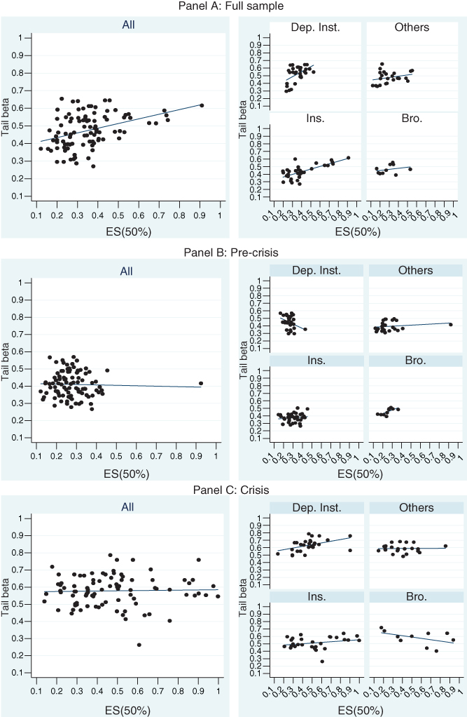
Figure 13.5 Tail risk (ES(X > 50%)) versus extreme systemic risk (tail-β) for full-sample, pre-crisis, and crisis.
Table 13.6 Rank correlation of tail risk and systemic risk with different proxies for size
| Total market capitalization | Total asset | Total equity | Total debt | |||||||||
| Full sample | Pre crisis | crisis | Full sample | Pre crisis | Crisis | Full sample | Pre crisis | Crisis | Full sample | Pre crisis | Crisis | |
| Panel A: q (p = 0.1%) | ||||||||||||
| Depositors | 11.2 | −1.1 | −11.9 | 18.6 | 1.0 | 39.1* | 16.4 | −1.6 | 35.2 | 19.2 | −3.8 | 29.8 |
| Others | 2.6 | 0.3 | −36.4 | −4.8 | −27.2 | −3.2 | −11.4 | −23.7 | −24.2 | −9.9 | −41.7* | 9.0 |
| Insurances | −6.1 | −20.6 | −22.2 | 30.4* | −7.4 | 42.9** | 10.2 | −14.7 | 8.6 | 6.0 | −20.4 | 8.8 |
| B&Ds | 32.1 | 28.5 | −32.1 | 37.0 | 27.3 | 48.6 | 25.0 | 15.0 | 48.6 | 36.7 | 26.7 | 40.0 |
| All | 4.0 | −1.9 | −19.3* | 20.7** | −3.1 | 43.8*** | 7.7 | −10.0 | 18.5* | 9.1 | −11.2 | 28.4** |
| Panel B: ES(X > 50%) | ||||||||||||
| Depositors | 20.3 | −15.1 | 21.8 | 23.7 | −17.1 | 51.5*** | 23.8 | −22.6 | 41.1 | 29.4 | −14.9 | 44.8 |
| Others | 11.3 | 16.2 | −3.6 | 8.8 | −1.2 | 17.0 | 14.8 | 13.3 | −5.7 | −1.4 | −7.7 | 0.8 |
| Insurances | 15.0 | −4.7 | −4.0 | 42.3** | 19.5 | 35.4* | 19.9 | 3.8 | 12.7 | 10.6 | −10.5 | −1.2 |
| B&Ds | 47.9 | 62.4* | −3.6 | 49.1 | 50.3 | 71.4 | 30.0 | 31.7 | 71.4 | 48.3 | 48.3 | 70.0 |
| All | 19.0* | 10.7 | 5.2 | 36.0*** | 14.5 | 41.2*** | 23.8** | 12.0 | 23.8** | 21.5** | 2.8 | 20.5* |
| Panel C: Tail-β | ||||||||||||
| Depositors | 68.7*** | 77.6*** | 67.2*** | 80.0*** | 81.4*** | 91.6*** | 78.9*** | 77.0*** | 88.6*** | 76.3*** | 76.9*** | 81.4*** |
| Others | 30.9 | 48.1** | −3.8 | 20.8 | 53.6** | 10.3 | 28.9 | 48.5** | 8.5 | 29.7 | 45.0** | 20.7 |
| Insurances | 11.6 | 34.9** | 7.0 | 45.4*** | 47.6*** | 32.2* | 27.4 | 30.8* | 14.7 | 21.9 | 32.6* | 2.5 |
| B&Ds | 59.0* | 76.6*** | 39.3 | 67.5** | 55.3* | −8.6 | 77.0** | 41.8 | −8.6 | 64.4* | 47.7 | 60.0 |
| All | 36.1*** | 50.9*** | 23.4** | 50.7*** | 55.9*** | 41.7*** | 43.9*** | 44.6*** | 32.7*** | 48.7*** | 53.1*** | 42.4*** |
Note: The table reports Spearman's rank correlation coefficients between a risk measure and a size proxy and the independence t-test. The test is carried across four industry groups separately and for all institution as a whole. The test is also carried across time dimension over full-sample, pre-crisis, and crisis period. The null-hypothesis rejections at the 10%, 5%, and 1% significance level are denoted with *, **, and ***, respectively.
13.5 Conclusions
The financial sector maintains a central role in every economy as creator of money and a transmitter of monetary policy, but they are also strongly involved in the multilateral payment system and finance investment and growth in the real sector. Thus, long-term financial stability, both for individual financial institutions (tail risk) and for the system as a whole (systemic risk), is of utmost importance for regulators and supervisors. In this study, we used techniques from statistical extreme value analysis to estimate a downside risk measure (per individual institution) and a systemwide risk measure (systemic risk). Both are market-based indicators: they use the loss tails of the market value of equity capital as an input. The downside risk is measured using an extreme tail quantile estimator, whereas the systemic risk is measured by the so-called co-crash probability of an individual bank stock together with a banking market index, that is, a so-called tail-β. Tail-βs are estimated by the so-called Ledford and Tawn approach.
We compare tail risk and systemic risk outcomes across four different industry groups containing 91 financial institutions as in Acharya et al. (2011) and Brownlees and Engle (2015): depositors, insurances, B&Ds, and others. This enables one to make cross-industry tail risk and systemic risk comparisons, which constitutes the main objective of this chapter. First, we find that different groups of financial institutions exhibit different levels of tail risk as well as systemic risk. Insurance companies exhibit the highest equity tail risk. Second, industry groups exhibiting the highest tail risk not necessarily contribute the most to the risk of the financial system as a whole. Somewhat surprisingly, deposit banks (and not B&Ds) seem to be most strongly exposed to adverse macro shocks. Third, both tail risk and systemic risk have increased over the crisis, which does not come as a surprise. However, the relative ranking of the financial institutions' riskiness is not changing dramatically over time: extreme systematic risk seems to exhibit some predictability toward future distress, as the rank correlations between pre-crisis and crisis tail-βs are found to be relatively high. Finally, institutional size proxies are not strongly correlated with tail risk (no diversification effect for larger institutions); but size seems to be correlated with our systemic risk measure. However, the size and ranking results vary considerably across industries and across time.
References
- Acharya, V., Pedersen, L., Philippon, T., Richardson, M. Measuring Systemic Risk. Working Paper, New York University; 2011.
- Adrian, T., Brunnermeier, M.K. CoVaR. NBER. Working Paper nr. 17454; 2011.
- Allen, F., Gale, D. Financial contagion. J Polit Econ 2000;108(1):1–33.
- Beirlant, J., Dierckx, G., Goegebeur, Y., Matthys, G. Tail index estimation and an exponential regression model. Extremes 1999;2(2):177–200.
- Brownlees, C.T., Engle, R. SRISK: a conditional capital shortfall measure of systemic risk. Working Paper; 2015.
- Demirgüc-Kunt, A., Detragiache, E. The determinants of banking crises in developing and developed countries. IMF Staff Pap 1998;45(1):81–109.
- De Haan, L., Jansen, D.W., Koedijk, K., de Vries, C.G. Safety first portfolio selection, extreme value theory and long run asset risks. In: Galambos, J., Lechner, J., Simiu, E., editors. Extreme Value Theory and Applications. Dordrecht: Kluwer Academic Publishers; 1994. p 471–487.
- De Jonghe, O. Back to basics in banking? A micro-analysis of banking system stability. J Financ Intermed 2010;19:387–417.
- De Nicolo, G., Kwast, M. Systemic risk and financial consolidation: Are they related? J Bank Financ 2002;26:861–880.
- De Vries, C.G. The simple economics of bank fragility. J Bank Financ 2005;29:803–825.
- Embrechts, P., Klüppelberg, C., Mikosch, T. Modelling Extremal Events. Berlin: Springer-Verlag; 1997.
- Goldie, C., Smith, R. Slow variation with remainder: theory and applications. Quart J Math 1987;38:45–71.
- Gonzalez-Hermosillo, B., Pazarbasioglu, C., Billings, R. Banking system fragility: likelihood versus timing of failure – an application to the Mexican financial crisis'. IMF Staff Pap 1997;44(3):295–314.
- Gorton, G. Banking panics and business cycles. Oxf Econ Pap 1988;40:751–781.
- Gropp, R., Moerman, G. Measurement of contagion in banks' equity prices. In: Hasan, I., Tarkka, J., editors. Banking, Development and Structural Change, Special Issue of the J Int Money Financ; 23(3): 2004. p 405–459.
- Gropp, R., Vesala, J., 2004. Bank contagion in Europe. Paper presented at the Symposium of the ECB-CFS Research Network on `Capital Markets and Financial Integration in Europe'; 10–11 May; Frankfurt am Main: European Central Bank.
- Haeusler, E., Teugels, J. On asymptotic normality of Hill's estimator for the exponent of regular variation. Ann Stat 1985;13:743–756.
- Harrington, S.E. The Financial Crisis, Systemic Risk, and the Future of Insurance Regulation, Public Policy Paper. National Association of Mutual Insurance Companies; 2009.
- Hartmann, P., Straetmans, S., de Vries, C.G. Banking System stability: a cross-atlantic perspective. In: Carey, M., Stulz, R.M., editors. The Risk of Financial Institutions. Chicago and London: The University of Chicago Press; 2006. p 133–193.
- Hellwig, M. Liquidity provision, banking, and the allocation of interest rate risk. Eur Econ Rev 1994;38(7):1363–1389.
- Hill, B.M. A simple general approach to inference about the tail of a distribution. Ann Stat 1975;3(5):1163–1173.
- Iori, G., Jafarey, S., Padilla, F. Systemic risk on the interbank market. J Behav Org 2006;61(4):525–542.
- Jansen, D.W., de Vries, C.G. On the frequency of large stock returns: putting booms and busts into perspective. Rev Econ Stat 1991;73:19–24.
- Kho, B.-C., Lee, D., Stulz, R. U.S. banks, crises, and bailouts: from Mexico to LTCM. Am Econ Rev Pap Proc 2000;90(2):28–31.
- Ledford, A., Tawn, J. Statistics for near independence in multivariate extreme values. Biometrika 1996;83(1):169–187.
- Mandelbrot, B. The variation of certain speculative prices. J Bus 1963;36:394–419.
- Slovin, M., Sushka, M., Polonchek, J. An analysis of contagion and competitive effects at commercial banks. J Financ Econ 1999;54:197–225.
- Smirlock, M., Kaufold, H. Bank foreign lending, mandatory disclosure rules, and the reaction of bank stock prices to the Mexican debt crisis. J Bus 1987;60(3):347–364.
- Straetmans, S., Verschoor, W., Wolff, C. Extreme US stock market fluctuations in the wake of 9/11. J Appl Econ 2008;23(1):17–42.
- Straetmans, S., Chaudhry, S. Tail risk and systemic risk for U.S. and Eurozone financial institutions in the wake of the global financial crisis. J Int Money Financ 2015;58:191–223.
- Swary, I. Stock market reaction to regulatory action in the Continental Illinois crisis. J Bus 1986;59(3):451–473.
- Tarashev, N., Borio, C., Tsatsaronis, K., 2010. Attributing systemic risk to individual institutions. BIS Working Paper nr. 308.
- Wall, L., Peterson, D. The effect of Continental Illinois' failure on the financial performance of other banks. J Monetary Econ 1990;26:77–79.
- Zhou, C. Are banks too big to fail? Measuring systemic importance of financial institutions. Int J Cent Bank 2010;6(4):205–250.
Appendix A
Table A1 Tail risk and systemic risk for deposit banks
| Full sample | Pre-crisis | Crisis | ||||||||||||||||
| α | q (p = 0.1%) | ES(X > 50%) | ES(p = 5%) | MES(p = 5%) | Tail-β | α | q (p = 0.1%) | ES(X > 50%) | ES(95%) | MES(95%) | Tail-β | α | q (p = 0.1%) | ES(X > 50%) | ES(95%) | MES(95%) | Tail-β | |
| Bank of America | 2.1 | 22.9 | 45.8 | 6.5 | 4.0 | 64.5 | 4.0 | 13.7 | 16.7 | 4.3 | 2.2 | 56.7 | 1.6 | 82.5 | 90.2 | 13.2 | 8.3 | 75.9 |
| BB&T | 2.9 | 12.5 | 25.9 | 4.9 | 3.4 | 56.7 | 3.1 | 8.9 | 23.8 | 3.6 | 1.6 | 44.9 | 2.6 | 23.7 | 31.6 | 8.2 | 7.1 | 66.7 |
| Bank of N.Y. MEL. | 2.6 | 15.2 | 30.5 | 5.5 | 3.4 | 54.5 | 3.1 | 10.8 | 23.6 | 4.5 | 2.1 | 53.6 | 2.1 | 33.2 | 47.0 | 8.8 | 6.8 | 65.4 |
| Citigroup | 2.1 | 23.4 | 43.5 | 6.9 | 3.9 | 64.5 | 2.7 | 12.5 | 28.6 | 4.5 | 2.2 | 56.9 | 1.8 | 66.5 | 66.5 | 14.0 | 7.7 | 70.3 |
| COM.BANC. | 2.9 | 14.1 | 26.7 | 5.3 | 0.9 | 30.8 | 3.0 | 13.9 | 25.4 | 5.4 | 0.9 | 29.7 | 4.6 | 5.9 | 13.9 | 3.0 | 2.5 | 51.7 |
| Comerica | 2.4 | 16.5 | 36.7 | 5.3 | 3.8 | 61.2 | 3.0 | 9.1 | 25.4 | 3.6 | 2.2 | 52.4 | 2.0 | 38.9 | 48.3 | 9.7 | 7.6 | 68.1 |
| HUNTINGTON BCSH. | 2.2 | 25.2 | 43.4 | 7.2 | 3.3 | 55.1 | 3.3 | 9.2 | 21.6 | 3.9 | 1.8 | 44.1 | 2.0 | 59.9 | 50.8 | 15.1 | 6.8 | 60.6 |
| HUDSON CITY BANC | 2.3 | 14.3 | 39.4 | 4.4 | 3.8 | 47.9 | 2.2 | 10.0 | 43.1 | 2.7 | 1.2 | 35.5 | 2.1 | 24.6 | 46.4 | 6.4 | 6.6 | 60.6 |
| JP Morgan C&CO. | 2.8 | 15.1 | 27.8 | 5.7 | 3.9 | 63.9 | 3.2 | 11.5 | 23.1 | 4.8 | 2.2 | 55.1 | 2.1 | 33.9 | 46.5 | 8.9 | 8.2 | 78.6 |
| KEYCORP | 2.3 | 20.0 | 38.9 | 6.3 | 3.7 | 60.6 | 2.9 | 9.8 | 26.5 | 3.7 | 2.1 | 50.3 | 2.0 | 48.1 | 48.1 | 12.7 | 7.8 | 69.5 |
| MARSHALL & ILSLEY | 2.3 | 20.1 | 38.3 | 6.3 | 3.4 | 57.4 | 3.6 | 7.6 | 19.1 | 3.4 | 1.8 | 44.9 | 2.0 | 50.1 | 49.5 | 13.1 | 7.2 | 61.6 |
| M&T BK. | 2.3 | 13.4 | 38.4 | 4.1 | 3.5 | 52.8 | 2.8 | 7.0 | 27.2 | 2.7 | 1.6 | 41.3 | 2.3 | 25.6 | 38.1 | 7.5 | 7.3 | 64.1 |
| NATIONAL CITY | 1.9 | 20.9 | 52.9 | 5.9 | 2.8 | 54.8 | 2.7 | 10.0 | 30.3 | 3.5 | 2.0 | 54.9 | 1.6 | 124.6 | 90.2 | 23.8 | 7.6 | 56.3 |
| NORTHERN TRUST | 2.8 | 12.6 | 27.1 | 4.9 | 3.4 | 54.2 | 2.9 | 10.4 | 26.1 | 4.0 | 2.1 | 50.0 | 2.0 | 32.1 | 52.1 | 7.7 | 6.5 | 64.1 |
| NY.CMTY.BANC. | 3.1 | 12.1 | 24.0 | 4.8 | 2.7 | 39.5 | 3.1 | 9.7 | 23.3 | 4.0 | 1.2 | 34.5 | 2.7 | 18.7 | 28.9 | 6.8 | 6.1 | 57.4 |
| PEOPLES UNITED FIN. | 2.7 | 15.3 | 28.8 | 5.6 | 1.6 | 31.9 | 2.6 | 16.3 | 31.4 | 5.7 | 0.5 | 29.6 | 2.3 | 17.2 | 37.6 | 5.3 | 6.4 | 55.1 |
| PNC FINL.SVS.GP. | 2.6 | 14.4 | 30.6 | 5.2 | 3.6 | 59.4 | 3.0 | 10.1 | 25.6 | 4.0 | 2.0 | 50.0 | 2.2 | 31.4 | 42.9 | 9.0 | 7.2 | 68.1 |
| REGIONS FINL.NEW | 2.0 | 24.9 | 48.6 | 6.8 | 3.5 | 59.0 | 2.8 | 10.1 | 28.0 | 3.7 | 1.7 | 44.9 | 1.9 | 63.2 | 57.2 | 14.0 | 6.9 | 64.1 |
| SYNOVUS FINL. | 2.3 | 21.5 | 38.5 | 6.7 | 3.1 | 48.7 | 3.3 | 9.0 | 21.5 | 3.9 | 1.7 | 45.6 | 2.5 | 40.0 | 34.5 | 12.7 | 5.8 | 55.1 |
| SOVEREIGN BANCORP | 2.5 | 19.1 | 32.8 | 7.0 | 2.0 | 39.3 | 2.8 | 14.2 | 27.7 | 5.2 | 1.0 | 32.4 | 1.5 | 130.8 | 102.5 | 21.0 | 8.5 | 60.2 |
| SUNTRUST BANKS | 2.7 | 17.7 | 30.2 | 5.9 | 3.8 | 64.1 | 3.5 | 7.5 | 19.9 | 3.4 | 2.1 | 54.0 | 2.5 | 34.4 | 33.6 | 11.7 | 7.5 | 66.7 |
| STATE STREET | 2.5 | 17.0 | 33.9 | 6.0 | 3.3 | 54.5 | 2.6 | 12.8 | 30.7 | 4.5 | 2.0 | 48.6 | 1.9 | 40.3 | 52.7 | 10.8 | 6.9 | 66.1 |
| UNIONBANCAL | 3.1 | 11.3 | 24.0 | 4.6 | 1.6 | 35.9 | 2.8 | 12.0 | 27.3 | 4.6 | 1.3 | 34.4 | 2.7 | 14.4 | 29.2 | 4.9 | 4.1 | 50.2 |
| US BANCORP | 2.5 | 15.1 | 32.9 | 5.2 | 3.4 | 53.2 | 3.1 | 10.1 | 24.1 | 4.1 | 1.6 | 43.9 | 1.9 | 39.1 | 57.7 | 8.7 | 8.0 | 75.9 |
| WACHOVIA | 2.1 | 19.9 | 44.6 | 6.3 | 3.0 | 58.5 | 2.8 | 10.8 | 28.0 | 3.9 | 2.1 | 52.9 | 1.5 | 139.3 | 100.4 | 25.1 | 8.4 | 66.8 |
| WELLS FARGO & CO | 2.4 | 16.2 | 35.6 | 5.3 | 3.8 | 61.2 | 2.9 | 9.7 | 25.9 | 3.7 | 2.0 | 48.3 | 2.0 | 39.7 | 49.8 | 9.9 | 8.2 | 75.9 |
| WASTE MAN. | 3.1 | 12.0 | 23.3 | 5.1 | 1.2 | 29.5 | 3.0 | 12.9 | 25.3 | 5.2 | 0.6 | 29.8 | 2.7 | 11.8 | 29.2 | 4.2 | 4.6 | 49.3 |
| WESTERN UNION | 2.3 | 19.5 | 38.9 | 5.9 | 5.1 | 49.7 | 2.6 | 10.1 | 30.7 | 3.3 | 0.8 | 42.3 | 2.2 | 22.5 | 42.5 | 6.3 | 5.4 | 49.7 |
| ZIONS BANCORP. | 2.1 | 23.4 | 44.4 | 6.6 | 3.2 | 53.5 | 2.6 | 11.9 | 31.2 | 4.2 | 1.3 | 36.8 | 2.2 | 44.2 | 41.2 | 12.3 | 6.8 | 63.5 |
Table A2 Tail risk and systemic risk for category “others”
| Full sample | Pre-crisis | Crisis | ||||||||||||||||
| α | q (p = 0.1%) | ES(X > 50%) | ES(95%) | MES(95%) | Tail-β | α | q (p = 0.1%) | ES(X > 50%) | ES(95%) | MES(95%) | Tail-β | α | q (p = 0.1%) | ES(X > 50%) | ES(95%) | MES(95%) | Tail-β | |
| AMERICAN CAPITAL | 2.2 | 30.4 | 40.8 | 9.2 | 3.4 | 46.3 | 2.4 | 15.7 | 36.1 | 5.0 | 1.0 | 33.8 | 2.2 | 52.4 | 42.3 | 15.3 | 5.7 | 58.5 |
| AMERIPRISE FINL. | 3.2 | 20.5 | 22.3 | 8.3 | 5.7 | 65.4 | 3.2 | 8.8 | 23.2 | 3.7 | 1.1 | 48.8 | 3.2 | 23.1 | 22.3 | 9.6 | 6.7 | 62.3 |
| TD AMERITRADE HOLDING | 3.5 | 21.2 | 20.1 | 9.3 | 2.3 | 37.3 | 3.6 | 21.6 | 19.3 | 9.7 | 1.2 | 39.4 | 2.0 | 29.4 | 50.3 | 7.5 | 6.9 | 59.0 |
| AMERICAN EXPRESS | 2.9 | 14.1 | 26.6 | 5.5 | 3.3 | 52.4 | 3.2 | 10.6 | 22.6 | 4.5 | 1.8 | 48.8 | 2.3 | 27.8 | 37.5 | 8.4 | 7.3 | 68.1 |
| FRANKLIN RESOURCES | 3.3 | 12.4 | 22.0 | 5.3 | 3.2 | 50.3 | 3.5 | 10.0 | 19.8 | 4.5 | 1.6 | 43.4 | 2.7 | 20.8 | 28.7 | 7.5 | 7.6 | 67.4 |
| BLACKROCK | 2.8 | 15.6 | 28.4 | 5.8 | 3.4 | 46.2 | 2.5 | 13.4 | 32.9 | 4.5 | 0.7 | 35.8 | 2.4 | 23.3 | 34.8 | 7.4 | 5.8 | 56.0 |
| CB RICHARD ELLIS GP. | 3.5 | 27.1 | 20.2 | 11.3 | 5.0 | 59.3 | 4.3 | 9.5 | 15.0 | 4.7 | 0.8 | 36.0 | 3.3 | 33.1 | 21.8 | 14.2 | 6.0 | 57.9 |
| COMPASS BANCSHARES | 5.1 | 6.9 | 12.1 | 3.7 | 1.5 | 37.0 | 5.1 | 6.9 | 12.1 | 3.7 | 1.5 | 36.9 | 1.9 | 17.0 | 56.5 | 2.9 | −1.3 | 58.3 |
| CIT GROUP | 1.9 | 71.6 | 55.1 | 18.8 | 4.0 | 56.7 | 2.6 | 13.3 | 32.1 | 4.6 | 1.3 | 49.4 | 2.1 | 109.5 | 44.2 | 33.7 | 4.6 | 51.2 |
| CME GROUP | 3.4 | 15.8 | 20.6 | 6.5 | 4.1 | 46.2 | 3.5 | 9.4 | 19.7 | 4.3 | 0.6 | 37.1 | 3.3 | 19.7 | 22.0 | 8.3 | 5.8 | 56.9 |
| CAPITAL ONE FINL | 2.4 | 24.1 | 35.5 | 8.0 | 3.7 | 53.2 | 2.4 | 19.8 | 34.7 | 6.6 | 1.9 | 47.3 | 2.0 | 46.6 | 52.0 | 11.4 | 7.0 | 67.4 |
| EATON VANCE NV. | 2.9 | 14.3 | 26.4 | 5.5 | 2.5 | 39.4 | 3.6 | 9.7 | 19.2 | 4.5 | 0.8 | 33.0 | 2.1 | 32.9 | 44.1 | 8.8 | 7.1 | 67.4 |
| FIDELITY NAT.INFO.SVS. | 2.8 | 12.2 | 27.5 | 4.7 | 3.5 | 39.8 | 2.6 | 11.3 | 30.8 | 4.2 | 1.2 | 38.2 | 2.7 | 15.0 | 29.9 | 5.3 | 5.1 | 50.8 |
| FIFTH THIRD BANCORP | 1.9 | 25.4 | 53.6 | 6.7 | 3.5 | 56.2 | 2.7 | 10.6 | 30.3 | 3.6 | 1.9 | 47.8 | 1.6 | 76.7 | 85.5 | 14.8 | 7.2 | 62.3 |
| INTERCONTINENTAL EX | 2.0 | 35.6 | 48.4 | 9.2 | 4.4 | 46.7 | 2.2 | 26.9 | 41.2 | 7.4 | 0.7 | 36.4 | 1.9 | 44.6 | 58.2 | 9.8 | 5.5 | 53.3 |
| JANUS CAPITAL GP. | 3.1 | 21.6 | 24.4 | 8.5 | 4.1 | 54.9 | 3.4 | 14.5 | 20.6 | 6.3 | 1.4 | 47.5 | 2.7 | 31.8 | 28.7 | 11.3 | 7.2 | 60.6 |
| LEGG MASON | 2.5 | 18.4 | 33.4 | 6.2 | 2.9 | 49.5 | 3.2 | 10.7 | 22.5 | 4.6 | 1.5 | 41.0 | 2.4 | 34.5 | 35.4 | 10.9 | 6.4 | 56.9 |
| LEUCADIA NATIONAL | 2.4 | 14.0 | 34.6 | 4.7 | 2.9 | 44.6 | 3.3 | 7.3 | 21.4 | 3.2 | 1.1 | 34.4 | 2.4 | 26.6 | 35.4 | 8.6 | 6.5 | 58.5 |
| MASTERCARD | 2.3 | 22.0 | 39.3 | 6.4 | 5.1 | 46.7 | 1.5 | 37.9 | 92.4 | 5.3 | 0.5 | 41.6 | 2.2 | 23.7 | 40.8 | 6.7 | 6.2 | 48.2 |
| NYSE EURONEXT | 3.5 | 18.1 | 20.1 | 7.7 | 4.7 | 54.0 | 4.6 | 9.7 | 13.8 | 5.2 | 0.5 | 33.6 | 3.4 | 21.5 | 20.7 | 9.2 | 6.8 | 61.7 |
| SEI INVESTMENTS | 3.9 | 13.0 | 17.1 | 5.8 | 2.4 | 35.9 | 3.2 | 13.1 | 22.4 | 5.4 | 1.2 | 31.1 | 3.3 | 16.6 | 21.8 | 7.0 | 6.6 | 61.2 |
| SLM | 2.0 | 25.9 | 50.4 | 6.9 | 2.6 | 42.9 | 2.8 | 10.9 | 27.0 | 4.2 | 1.0 | 33.3 | 1.9 | 63.1 | 56.5 | 14.4 | 5.9 | 55.5 |
| UNION PACIFIC | 4.2 | 8.3 | 15.6 | 4.0 | 2.4 | 36.9 | 4.8 | 6.3 | 13.3 | 3.3 | 1.0 | 32.2 | 4.4 | 11.5 | 14.8 | 6.0 | 6.4 | 56.0 |
Table A3 Tail risk and systemic risk for insurance companies
| Full sample | Pre-crisis | Crisis | ||||||||||||||||
| α | q (p = 0.1%) | ES(X > 50%) | ES(95%) | MES(95%) | Tail-βa | α | q (p = 0.1%) | ES(X > 50%) | ES(95%) | MES(95%) | Tail-β | α | q (p = 0.1%) | ES(X > 50%) | ES(95%) | MES(95%) | Tail-β | |
| AETNA | 2.3 | 16.6 | 37.4 | 5.3 | 2.0 | 36.2 | 2.3 | 15.1 | 38.1 | 4.8 | 1.0 | 34.5 | 1.9 | 30.5 | 53.8 | 7.0 | 4.5 | 45.9 |
| AFLAC | 2.2 | 17.6 | 40.4 | 5.4 | 2.8 | 42.7 | 2.7 | 11.5 | 29.9 | 4.0 | 1.3 | 38.8 | 1.4 | 73.0 | 113.2 | 10.0 | 6.2 | 59.0 |
| AMERICAN INTL.GP. | 1.7 | 35.3 | 74.3 | 7.8 | 3.2 | 53.3 | 2.5 | 11.1 | 33.0 | 3.6 | 1.9 | 43.4 | 1.4 | 130.2 | 111.2 | 19.3 | 4.7 | 56.5 |
| ASSURANT | 1.7 | 31.5 | 73.6 | 6.4 | 4.9 | 56.0 | 2.2 | 9.3 | 40.1 | 2.7 | 0.8 | 37.6 | 1.6 | 51.4 | 88.3 | 8.4 | 6.8 | 55.1 |
| ALLSTATE | 2.2 | 17.3 | 42.6 | 5.1 | 2.9 | 42.3 | 2.5 | 12.4 | 34.4 | 4.0 | 1.5 | 38.4 | 1.5 | 54.3 | 99.7 | 8.1 | 6.6 | 54.6 |
| AON | 2.3 | 13.4 | 37.5 | 4.4 | 2.2 | 41.1 | 2.2 | 14.3 | 41.7 | 4.4 | 1.4 | 39.5 | 2.0 | 18.7 | 50.5 | 4.3 | 5.3 | 52.4 |
| W R BERKLEY | 3.5 | 8.9 | 20.0 | 3.9 | 1.9 | 29.5 | 3.6 | 7.8 | 19.1 | 3.6 | 0.9 | 28.7 | 3.4 | 11.7 | 20.7 | 5.1 | 5.7 | 46.5 |
| BERKSHIRE HATHAWAY A' | 2.7 | 9.5 | 28.6 | 3.5 | 1.9 | 33.5 | 2.5 | 9.5 | 32.5 | 3.2 | 0.8 | 30.5 | 2.6 | 12.8 | 31.9 | 4.4 | 5.2 | 46.5 |
| BERKSHIRE HATHAWAY B' | 3.0 | 8.9 | 25.3 | 3.5 | 2.6 | 37.1 | 2.9 | 7.8 | 26.1 | 3.0 | 1.0 | 33.8 | 2.4 | 14.1 | 35.2 | 4.4 | 5.8 | 48.9 |
| CHUBB | 3.6 | 8.9 | 19.6 | 3.8 | 2.8 | 44.1 | 4.0 | 7.0 | 16.6 | 3.4 | 1.7 | 41.3 | 3.1 | 14.5 | 23.7 | 5.7 | 6.6 | 59.5 |
| COUNTRYWIDE FINL. | 3.0 | 15.3 | 25.1 | 6.1 | 1.1 | 39.5 | 3.4 | 11.8 | 21.0 | 5.2 | 0.4 | 35.9 | 1.8 | 37.5 | 60.8 | 8.3 | 4.1 | 26.3 |
| LOEWS | 2.3 | 13.0 | 38.3 | 4.1 | 2.8 | 44.9 | 2.6 | 9.4 | 31.8 | 3.2 | 1.2 | 36.6 | 1.6 | 42.2 | 83.3 | 7.0 | 6.8 | 64.1 |
| CIGNA | 2.3 | 16.3 | 38.1 | 5.2 | 2.2 | 40.1 | 2.4 | 12.8 | 35.1 | 4.3 | 1.0 | 34.8 | 1.8 | 38.1 | 59.2 | 8.3 | 5.3 | 50.4 |
| CINCINNATI FINL. | 3.1 | 10.6 | 24.3 | 4.3 | 2.8 | 45.6 | 3.4 | 8.2 | 20.6 | 3.6 | 1.3 | 37.0 | 2.3 | 20.6 | 38.1 | 6.4 | 6.7 | 62.3 |
| AMERICAN NAT | 2.2 | 15.5 | 40.3 | 4.8 | 2.9 | 41.8 | 2.9 | 8.8 | 26.0 | 3.4 | 1.4 | 36.3 | 1.7 | 49.8 | 75.9 | 9.4 | 6.5 | 58.5 |
| COVENTRY HEALTH CARE | 2.3 | 26.6 | 37.8 | 8.7 | 1.1 | 27.0 | 2.3 | 27.0 | 37.8 | 8.6 | 0.4 | 26.6 | 1.8 | 37.2 | 63.5 | 8.6 | 4.1 | 43.5 |
| FIDELITY NAT.FINANCIAL | 2.5 | 21.1 | 33.5 | 7.1 | 4.1 | 44.5 | 2.5 | 12.1 | 34.1 | 4.0 | 0.6 | 38.5 | 2.3 | 26.9 | 39.4 | 7.9 | 5.2 | 48.6 |
| GENWORTH FINANCIAL | 2.5 | 44.2 | 32.9 | 13.7 | 4.6 | 59.9 | 4.4 | 5.6 | 14.5 | 2.8 | 0.9 | 41.5 | 2.8 | 51.3 | 28.0 | 18.3 | 5.5 | 55.1 |
| HARTFORD FINL.SVS.GP. | 1.7 | 36.9 | 68.5 | 8.4 | 3.5 | 51.5 | 2.3 | 15.6 | 39.8 | 4.3 | 1.9 | 42.6 | 1.3 | 150.9 | 166.5 | 17.3 | 5.8 | 53.7 |
| HEALTH NET | 2.8 | 17.5 | 28.2 | 6.5 | 1.5 | 31.1 | 2.7 | 17.0 | 29.7 | 6.1 | 0.8 | 29.9 | 1.9 | 31.2 | 54.1 | 7.6 | 3.7 | 41.3 |
| HUMANA | 2.4 | 19.8 | 35.4 | 6.6 | 1.6 | 31.6 | 2.3 | 20.3 | 37.3 | 6.3 | 0.7 | 29.6 | 1.9 | 29.2 | 52.8 | 7.3 | 5.3 | 43.7 |
| LINCOLN NAT. | 1.8 | 29.7 | 65.1 | 6.9 | 3.1 | 51.6 | 2.3 | 13.4 | 37.9 | 3.9 | 1.7 | 41.9 | 1.3 | 157.0 | 185.0 | 15.4 | 7.0 | 62.3 |
| MBIA | 2.4 | 27.2 | 36.6 | 8.4 | 2.8 | 45.9 | 2.9 | 10.5 | 26.5 | 4.1 | 1.4 | 38.9 | 2.7 | 47.8 | 29.9 | 17.0 | 6.0 | 49.7 |
| METLIFE | 1.9 | 28.6 | 55.9 | 7.1 | 4.2 | 54.6 | 2.6 | 11.4 | 31.1 | 3.8 | 1.5 | 44.7 | 1.6 | 65.3 | 84.2 | 11.3 | 6.8 | 55.5 |
| MARSH & MCLENNAN | 2.9 | 10.2 | 26.4 | 4.0 | 2.6 | 43.7 | 3.0 | 9.3 | 25.0 | 3.8 | 1.6 | 42.2 | 2.3 | 16.1 | 38.7 | 4.8 | 5.8 | 56.0 |
| PRINCIPAL FINL.GP. | 1.7 | 41.5 | 72.6 | 8.6 | 4.6 | 58.7 | 2.4 | 10.7 | 34.8 | 3.3 | 1.5 | 50.3 | 1.5 | 89.0 | 97.5 | 13.2 | 7.3 | 60.6 |
| PROGRESSIVE OHIO | 2.4 | 13.5 | 36.0 | 4.4 | 2.6 | 41.1 | 2.5 | 11.5 | 33.3 | 3.9 | 1.3 | 38.3 | 1.7 | 32.7 | 68.6 | 6.0 | 6.9 | 59.5 |
| PRUDENTIAL FINL. | 1.5 | 45.9 | 91.0 | 8.3 | 4.7 | 61.6 | 2.1 | 12.7 | 45.5 | 3.2 | 1.7 | 49.1 | 1.4 | 105.4 | 133.8 | 12.9 | 6.9 | 61.7 |
| SAFECO | 3.1 | 8.9 | 23.6 | 3.7 | 1.5 | 37.7 | 3.0 | 9.2 | 24.9 | 3.7 | 1.3 | 38.0 | 2.8 | 11.1 | 28.1 | 3.9 | 2.8 | 46.8 |
| TORCHMARK | 2.4 | 13.8 | 36.3 | 4.5 | 3.0 | 49.4 | 2.8 | 9.5 | 28.5 | 3.5 | 1.6 | 42.1 | 1.7 | 40.5 | 69.4 | 8.0 | 6.4 | 59.0 |
| TRAVELERS COS. | 3.5 | 9.8 | 20.0 | 4.2 | 2.8 | 41.9 | 3.9 | 7.9 | 17.0 | 3.6 | 1.5 | 39.2 | 2.7 | 16.6 | 29.4 | 6.0 | 6.9 | 57.4 |
| UNITEDHEALTH GP. | 2.7 | 15.9 | 29.5 | 5.9 | 1.5 | 28.7 | 2.8 | 14.6 | 27.4 | 5.6 | 0.7 | 27.8 | 2.0 | 26.8 | 49.8 | 6.8 | 4.5 | 45.9 |
| UNUM GROUP | 2.0 | 23.1 | 50.8 | 6.3 | 2.9 | 47.1 | 2.2 | 17.2 | 42.7 | 5.3 | 1.4 | 37.6 | 1.5 | 67.2 | 101.9 | 9.4 | 7.0 | 62.3 |
| WELLPOINT | 3.0 | 12.7 | 25.4 | 5.1 | 2.9 | 39.6 | 3.0 | 10.7 | 25.4 | 4.2 | 0.8 | 31.1 | 2.8 | 15.6 | 27.4 | 6.1 | 4.9 | 44.6 |
Table A4 Tail risk and systemic risk measures for “Broker-dealers”
| Full sample | Pre-crisis | Crisis | ||||||||||||||||
| α | q (p = 0.1%) | ES(X > 50%) | ES(95%) | MES(95%) | Tail-β | α | q (p = 0.1%) | ES(X > 50%) | ES(95%) | MES(95%) | Tail-β | α | q (p = 0.1%) | ES(X > 50%) | ES(95%) | MES(95%) | Tail-β | |
| A G EDWARDS | 3.7 | 9.4 | 18.2 | 4.4 | 1.6 | 41.7 | 3.7 | 9.4 | 18.3 | 4.4 | 1.6 | 41.6 | 3.8 | 4.1 | 17.8 | 1.9 | 1.2 | 71.9 |
| BEAR STEARNS | 2.9 | 13.3 | 26.7 | 5.9 | 2 | 45.2 | 3 | 11.8 | 24.6 | 4.7 | 1.8 | 44.2 | 1.5 | 85.2 | 93.8 | 28.7 | 2.6 | 55.3 |
| E*TRADE FINANCIAL | 3.2 | 27.2 | 23 | 11.3 | 2.6 | 41.2 | 3.1 | 24.2 | 24 | 9.7 | 1.1 | 39.2 | 2.3 | 46.5 | 38.1 | 14.9 | 6.1 | 54.6 |
| GOLDMAN SACHS GP. | 2.6 | 17 | 31 | 6 | 4 | 52.7 | 2.9 | 12.8 | 26.5 | 4.8 | 2 | 48.4 | 2 | 32.8 | 49.9 | 8 | 6.3 | 60.1 |
| LEHMAN BROS.HDG. | 1.9 | 42.7 | 53 | 12.2 | 2.3 | 46.4 | 2.4 | 19.2 | 36.5 | 5.9 | 2 | 48.3 | 1.7 | 117.2 | 75.9 | 26.3 | 3 | 40.3 |
| MERRILL LYNCH & CO. | 2.4 | 18.8 | 34.7 | 6.3 | 3 | 52.7 | 2.9 | 13.2 | 26.8 | 4.9 | 2 | 49.4 | 1.6 | 112.2 | 87.3 | 16.4 | 8 | 64.2 |
| MORGAN STANLEY | 2.5 | 21.3 | 34 | 7.2 | 3.7 | 55.4 | 2.7 | 15.2 | 28.7 | 5.5 | 2.1 | 51 | 1.7 | 56.4 | 67.4 | 11.7 | 7 | 64.1 |
| NYMEX HOLDINGS | 2.3 | 20.6 | 37.3 | 6.5 | 1.6 | 38.9 | 2.6 | 13.7 | 30.7 | 4 | 0.9 | 49.1 | 1.8 | 40.9 | 65.8 | 7.8 | 1.1 | 44.2 |
| CHARLES SCHWAB | 3.5 | 14.8 | 20 | 6.7 | 2.7 | 40.8 | 3.4 | 15 | 21 | 6.6 | 1.7 | 41.6 | 2.4 | 23.6 | 35.1 | 7.2 | 6.5 | 59.5 |
| T ROWE PRICE GP. | 4 | 12.3 | 16.4 | 5.9 | 3 | 47.4 | 4.4 | 10.1 | 14.6 | 5.2 | 1.5 | 42.2 | 3.4 | 19.2 | 21 | 8.3 | 7.3 | 67.4 |