
Chapter 7
Extreme Values Statistics for Markov Chains with Applications to Finance and Insurance
Patrice Bertail1, Stéphan Clémençon2 and Charles Tillier1
1MODAL'X, Université Paris-Ouest, Nanterre, France
2TSI, TelecomParisTech, Paris, France
AMS 2000 Mathematics Subject Classification: 60G70, 60J10, 60K20.
7.1 Introduction
Extremal events for (strongly or weakly) dependent data have received an increasing attention in the statistical literature in the last past years (see (Newell, 1964); (Loynes, 1965); (O'Brien, 1974), (O'Brien, 1987); (Hsing, 1988), (Hsing, 1991), (Hsing, 1993); (Resnick and Stărică, 1995); (Rootzén, 2009), for instance). A major issue for evaluating risks and understanding extremes and their possible replications is to take into account some dependencies. Indeed, whereas extreme values naturally occur in an isolated fashion in the identically independent distributed (i.i.d.) setup, since extreme values may be highly correlated, they generally tend to take place in small clusters for weakly dependent sequences. Most methods for statistical analysis of extremal events in weakly dependent setting rely on (fixed length) blocking techniques, which consist, roughly speaking, in dividing an observed data series into (overlapping or nonoverlapping) blocks of fixed length. Examining how extreme values occur over these data segments allows to capture the tail and the dependency structure of extreme values.
As originally pointed out in Rootzén (1988), the extremal behavior of instantaneous functionals ![]() of a Harris recurrent Markov chain
of a Harris recurrent Markov chain ![]() may be described through the regenerative properties of the underlying chain. This chapter emphasizes the importance of renewal theory and regeneration from the perspective of statistical inference for extremal events. Indeed, as observed by Rootzén (1988) (see also (Asmussen, 1998a); (Asmussen, 1998b); (Haiman et al., 1995); (Hansen and Jensen, 2005)), certain parameters of extremal behavior features of Harris Markov chains may be also expressed in terms of regeneration cycles, namely, data segments between consecutive regeneration times
may be described through the regenerative properties of the underlying chain. This chapter emphasizes the importance of renewal theory and regeneration from the perspective of statistical inference for extremal events. Indeed, as observed by Rootzén (1988) (see also (Asmussen, 1998a); (Asmussen, 1998b); (Haiman et al., 1995); (Hansen and Jensen, 2005)), certain parameters of extremal behavior features of Harris Markov chains may be also expressed in terms of regeneration cycles, namely, data segments between consecutive regeneration times ![]() , that is, random times at which the chain completely forgets its past. Following in the footsteps of the seminal contribution of Rootzén (1988) (see also (Asmussen, 1998a)), Bertail et al. (2009) and Bertail et al. (2013) have recently investigated the performance of regeneration-based statistical procedures for estimating key parameters, related to the extremal behavior analysis in a Markovian setup. In the spirit of the works of Bertail and Clémençon (2006b) (refer also to (Bertail and Clémençon, 2004a); (Bertail and Clémençon, 2004b); (Bertail and Clémençon, 2006a)), they developed a statistical methodology, called the “pseudoregenerative method,” based on approximating the pseudoregeneration properties of general Harris Markov chains, for tackling various estimation problems in a Markovian setup. Most of their works deal with regular differentiable functionals like the mean (see (Bertail and Clémençon, 2004a), (Bertail and Clémençon, 2007)), the variance, quantiles,
, that is, random times at which the chain completely forgets its past. Following in the footsteps of the seminal contribution of Rootzén (1988) (see also (Asmussen, 1998a)), Bertail et al. (2009) and Bertail et al. (2013) have recently investigated the performance of regeneration-based statistical procedures for estimating key parameters, related to the extremal behavior analysis in a Markovian setup. In the spirit of the works of Bertail and Clémençon (2006b) (refer also to (Bertail and Clémençon, 2004a); (Bertail and Clémençon, 2004b); (Bertail and Clémençon, 2006a)), they developed a statistical methodology, called the “pseudoregenerative method,” based on approximating the pseudoregeneration properties of general Harris Markov chains, for tackling various estimation problems in a Markovian setup. Most of their works deal with regular differentiable functionals like the mean (see (Bertail and Clémençon, 2004a), (Bertail and Clémençon, 2007)), the variance, quantiles, ![]() -statistics and their robustified versions (Bertail et al., 2015), as well as
-statistics and their robustified versions (Bertail et al., 2015), as well as ![]() -statistics (Bertail et al., 2011). Bootstrap versions of these estimates have also been proposed. For regular functionals, they possess the same nice second-order properties as the bootstrap in the i.i.d. case, that is, the rate of the convergence of the bootstrap distribution which is close to
-statistics (Bertail et al., 2011). Bootstrap versions of these estimates have also been proposed. For regular functionals, they possess the same nice second-order properties as the bootstrap in the i.i.d. case, that is, the rate of the convergence of the bootstrap distribution which is close to ![]() , for regular Markov chains, instead of
, for regular Markov chains, instead of ![]() for the asymptotic (Gaussian) benchmark (see (Bertail and Clémençon, 2006b)).
for the asymptotic (Gaussian) benchmark (see (Bertail and Clémençon, 2006b)).
The purpose of this chapter is to review and give some extensions of this approach in the framework of extreme values for general Markov chains. The proposed methodology consists in splitting up the observed sample path into regeneration data blocks (or into data blocks drawn from a distribution approximating the regeneration cycle's distribution, in the general case when regeneration times cannot be observed). We mention that the estimation principle exposed in this chapter is by no means restricted to the sole Markovian setup, but indeed applies to any process for which a regenerative extension can be constructed and simulated from available data (see Chapter 10 in Thorisson (2000)). Then, statistical tools are built over the sequence of maxima over the resulting data segments, as if these maxima were i.i.d. In order to illustrate the interest of this technique, we focus on the question of estimating the sample maximum's tail, the extremal dependence index, and the tail index by means of the (pseudo)regenerative method. To motivate this approach in financial and insurance applications (as well as queuing or inventory models), we illustrate how these tools may be used in order to estimate ruin probabilities or extremal index, in ruin models with a dividend barrier, exhibiting some regenerative properties. Such applications have also straightforward extensions (for continuous Markov chains) in the field of finance, for instance for put option pricing (for which the “strike” plays here the role of the ruin level).
7.2 On the (pseudo) Regenerative Approach for Markovian Data
Here and throughout, ![]() denotes a
denotes a ![]() -irreducible aperiodic time-homogeneous Markov chain, valued in a (countable generated) measurable space
-irreducible aperiodic time-homogeneous Markov chain, valued in a (countable generated) measurable space ![]() with transition probability
with transition probability ![]() and initial distribution
and initial distribution ![]() . We recall that the Markov property means that, for any set
. We recall that the Markov property means that, for any set ![]() , such that
, such that ![]() , for any sequence
, for any sequence ![]() in
in ![]() ,
,

For homogeneous Markov chains, the transition probability does not depend on ![]() . Refer to Revuz (1984) and Meyn and Tweedie (1996) for basic concepts of the Markov chain theory. For sake of completeness, we specify the two following notions:
. Refer to Revuz (1984) and Meyn and Tweedie (1996) for basic concepts of the Markov chain theory. For sake of completeness, we specify the two following notions:
- The chain is irreducible if there exists a
 -finite measure
  such that for all set
  , when
  , the chain visits
  with a strictly positive probability, no matter what the starting point.
 - Assuming
 -irreducibility, there are
  and disjointed sets
  ,
,  (
( ) weighted by
  such that
  and
and  ,
,  . The period of the chain is the greatest common divisor
  of such integers. It is aperiodic if
  .
. - The chain is said to be recurrent if any set
 with positive measure
  , if and only if (i.f.f.) the set
  is visited an infinite number of times.
The first notion formalizes the idea of a communicating structure between subsets, and the second notion considers the set of time points at which such communication may occur. Aperiodicity eliminates deterministic cycles. If the chain satisfies these three properties, it is said to be Harris recurrent.
In what follows, ![]() (respectively,
(respectively, ![]() for
for ![]() in
in ![]() ) denotes the probability measure on the underlying space such that
) denotes the probability measure on the underlying space such that ![]() (resp., conditioned upon
(resp., conditioned upon ![]() ),
), ![]() the
the ![]() -expectation (resp.
-expectation (resp. ![]() the
the ![]() -expectation), and
-expectation), and ![]() the indicator function of any event
the indicator function of any event ![]() . We assume further that
. We assume further that ![]() is positive recurrent and denote by
is positive recurrent and denote by ![]() its (unique) invariant probability distribution.
its (unique) invariant probability distribution.
7.2.1 Markov Chains with Regeneration Times: Definitions and Examples
A Markov chain ![]() is said regenerative when it possesses an accessible atom, that is, a measurable set
is said regenerative when it possesses an accessible atom, that is, a measurable set ![]() such that
such that ![]() and
and ![]() for all
for all ![]() ,
, ![]() in
in ![]() . A recurrent Markov chain taking its value in a finite set is always atomic since each visited point is itself an atom. Queuing systems or ruin models visiting an infinite number of time the value 0 (the empty queue) or a given level (for instance, a barrier in the famous Cramér–Lundberg model; see Embrechts et al. (1997) and the following examples) are also naturally atomic. Refer also to Asmussen (2003) for regenerative models involved in queuing theory, and see also the examples and the following applications.
. A recurrent Markov chain taking its value in a finite set is always atomic since each visited point is itself an atom. Queuing systems or ruin models visiting an infinite number of time the value 0 (the empty queue) or a given level (for instance, a barrier in the famous Cramér–Lundberg model; see Embrechts et al. (1997) and the following examples) are also naturally atomic. Refer also to Asmussen (2003) for regenerative models involved in queuing theory, and see also the examples and the following applications.
Denote then by ![]() the hitting time on
the hitting time on ![]() or first return time to
or first return time to ![]() . Put also
. Put also ![]() for the so-called successive return times to
for the so-called successive return times to ![]() , corresponding to the time of successive visits to the set
, corresponding to the time of successive visits to the set ![]() .
.
In the following ![]() denotes the expectation conditioned on the event
denotes the expectation conditioned on the event ![]() . When the chain is Harris recurrent, for any starting distribution, the probability of returning infinitely often to the atom
. When the chain is Harris recurrent, for any starting distribution, the probability of returning infinitely often to the atom ![]() is equal to one. Then, for any initial distribution
is equal to one. Then, for any initial distribution ![]() , by the strong Markov property, the sample paths of the chain may be divided into i.i.d. blocks of random length corresponding to consecutive visits to
, by the strong Markov property, the sample paths of the chain may be divided into i.i.d. blocks of random length corresponding to consecutive visits to ![]() , generally called regeneration cycles:
, generally called regeneration cycles:
taking their values in the torus ![]() . The renewal sequence
. The renewal sequence ![]() defines successive times at which the chain forgets its past, termed regeneration times.
defines successive times at which the chain forgets its past, termed regeneration times.
Example 1: Queuing system or storage process with an empty queue
We consider here a storage model (or a queuing system), evolving through a sequence of input times ![]() (with
(with ![]() by convention), at which the storage is refilled. Such models appear naturally in not only many domains like hydrology and operation research but also for modeling computer CPU occupancy.
by convention), at which the storage is refilled. Such models appear naturally in not only many domains like hydrology and operation research but also for modeling computer CPU occupancy.
Let ![]() be the size of the input into the storage system at time
be the size of the input into the storage system at time ![]() . Between each input time, it is assumed that withdrawals are done from the storage system at a constant rate
. Between each input time, it is assumed that withdrawals are done from the storage system at a constant rate ![]() . Then, in a time period
. Then, in a time period ![]() ,
, ![]() , the amount of stored contents which disappears is equal to
, the amount of stored contents which disappears is equal to ![]() . If
. If ![]() denotes the amount of contents immediately before the input time
denotes the amount of contents immediately before the input time ![]() , we have, for all
, we have, for all ![]() ,
,
with ![]() ,
, ![]() by convention and
by convention and ![]() for all
for all ![]() and
and ![]() is sometimes called the waiting time period.
is sometimes called the waiting time period.
This model can be seen as a reflected random walk on ![]() . Assume that, conditionally to
. Assume that, conditionally to ![]() ,
, ![]() , the amounts of input
, the amounts of input ![]() ,
, ![]() are independent from each other and independent from the interarrival times
are independent from each other and independent from the interarrival times ![]() ,
, ![]() and that the distribution of
and that the distribution of ![]() is given by
is given by ![]() for
for ![]() . Under the further assumption that
. Under the further assumption that ![]() is an i.i.d. sequence, independent from
is an i.i.d. sequence, independent from ![]() , the storage process
, the storage process ![]() is a Markov chain. The case with exponential input–output has been extensively studied in Asmussen (1998a).
is a Markov chain. The case with exponential input–output has been extensively studied in Asmussen (1998a).
It is known that the chain ![]() is irreducible as soon as
is irreducible as soon as ![]() has an infinite tail for all
has an infinite tail for all ![]() and if in addition
and if in addition ![]() ,
, ![]() is an accessible atom of the chain
is an accessible atom of the chain ![]() . Moreover, if
. Moreover, if ![]() has exponential tails, then the chain is exponentially geometrically ergodic. The case with heavy tails has been studied in detail by Asmussen (1998b) and Asmussen et al. (2000). Under some technical assumptions, the chain is recurrent positive, and the times at which the storage process
has exponential tails, then the chain is exponentially geometrically ergodic. The case with heavy tails has been studied in detail by Asmussen (1998b) and Asmussen et al. (2000). Under some technical assumptions, the chain is recurrent positive, and the times at which the storage process ![]() reaches the value 0 are regeneration times. This property allows to define regeneration blocks dividing the sample path into independent blocks, as shown in the following. Figure 7.1 represents the storage process with
reaches the value 0 are regeneration times. This property allows to define regeneration blocks dividing the sample path into independent blocks, as shown in the following. Figure 7.1 represents the storage process with ![]() and
and ![]() with
with ![]() distribution and
distribution and ![]() The horizontal line corresponds to the atom
The horizontal line corresponds to the atom ![]() and the vertical lines are the corresponding renewal times (visit to the atom).
and the vertical lines are the corresponding renewal times (visit to the atom).

Figure 7.1 Splitting a reflected random walk, with an atom at {0}; vertical lines corresponds to regeneration times, at which the chain forgets its past. A block is a set of observations between two lines (it may be reduced to {0} in some case).
Notice that the blocks are of random size. Some are rather long (corresponding to large excursion of the chain); others reduce to the point ![]() if the chain stays at 0 for several periods. In this example, for the given values of the parameters, the mean length of a block is close to 50.5. It is thus clear that we need a lot of observations to get enough blocks. The behavior of the maximum of this process for subexponential arrivals has been studied at length in Asmussen (1998b).
if the chain stays at 0 for several periods. In this example, for the given values of the parameters, the mean length of a block is close to 50.5. It is thus clear that we need a lot of observations to get enough blocks. The behavior of the maximum of this process for subexponential arrivals has been studied at length in Asmussen (1998b).
Example 2: Cramér–Lundberg with a dividend barrier
Ruin models, used in insurance, are dynamic models in continuous time which describe the behavior of the reserve of a company as a function of:
- Its initial reserve
 (which may be chosen by the insurer)
 - The claims which happen at some random times (described by a arrival claims process)
- The premium rate which is the price paid by customers per unit of time
In the classical Cramér–Lundberg model (Figure 7.2), the claims arrival process![]() is supposed to be an homogeneous Poisson process with rate
is supposed to be an homogeneous Poisson process with rate ![]() , modeling the number of claims in an interval
, modeling the number of claims in an interval ![]() . The claims sizes
. The claims sizes ![]() ,…,
,…,![]() , which an insurance company has to face, are assumed to be strictly positive and independent, with cumulative distribution function (c.d.f.)
, which an insurance company has to face, are assumed to be strictly positive and independent, with cumulative distribution function (c.d.f.) ![]() The premium rate is supposed to be constant equal to
The premium rate is supposed to be constant equal to ![]() Then, the total claims process, given by
Then, the total claims process, given by ![]()
![]() , is a compound Poisson process. Starting with an initial reserve
, is a compound Poisson process. Starting with an initial reserve ![]() , the reserve of the company evolves as
, the reserve of the company evolves as

One of the major problems in ruin models for insurance company is how to choose the initial amount to avoid the ruin or at least ensure that the probability of ruin over a finite horizon (or an infinite one) is small, equal to some given error of first kind, for instance, ![]() . The probability of ruin for an initial reserve
. The probability of ruin for an initial reserve ![]() over an horizon
over an horizon ![]() is given by
is given by
Notice that this model is very close to the queuing process considered in Example 1. The input times ![]() correspond here to the times of the claims. It is easy to see that under the given hypotheses, the interarrival times
correspond here to the times of the claims. It is easy to see that under the given hypotheses, the interarrival times ![]() are i.i.d. with exponential distribution
are i.i.d. with exponential distribution ![]() (with
(with ![]() . However, most of the time, for a given company, we only observe (at most) one ruin (since it is an absorbing state), and the reserve is not allowed to grow over a given barrier. Actually, if the process
. However, most of the time, for a given company, we only observe (at most) one ruin (since it is an absorbing state), and the reserve is not allowed to grow over a given barrier. Actually, if the process ![]() crosses a given threshold
crosses a given threshold ![]() , the money is redistributed in some way to the shareholders of the company. This threshold is called a dividend barrier. In this case the process of interest is rather 1
, the money is redistributed in some way to the shareholders of the company. This threshold is called a dividend barrier. In this case the process of interest is rather 1
where ![]() designs the infimum between
designs the infimum between ![]() and
and ![]() . Of course, the existence of a barrier reinforces the risk of ruin especially if the claims size may be large in particular if their distributions have a fat tail. The embedded chain is defined as the value of
. Of course, the existence of a barrier reinforces the risk of ruin especially if the claims size may be large in particular if their distributions have a fat tail. The embedded chain is defined as the value of ![]() at the claim times, say,
at the claim times, say, ![]() then it is easy to see that we have
then it is easy to see that we have

Figure 7.2 Cramér–Lundberg model with a dividend barrier at  (where the chain is reflected); ruin occurs at
  when the chain goes below 0.
Otherwise, the probability of no ruin is clearly linked to the behavior of ![]()
In comparison to Example 1, this model is simply a mirror process, with this time an atom at ![]() instead of
instead of ![]() as shown in the following two graphics. In this example, the
as shown in the following two graphics. In this example, the ![]() are exponential and the claims with exponential tails; the initial reserve is 5 and the barrier at 9. In this simulation the “ruin” is attained at time
are exponential and the claims with exponential tails; the initial reserve is 5 and the barrier at 9. In this simulation the “ruin” is attained at time ![]() .
.
The embedded chain shows that the barrier is attained several times and allows to build regeneration times (vertical lines) and independent blocks just as in the first example. Because of the choice of the parameters (fat tail for the claims), the number of blocks is small on this short period, but in practical insurance applications, we may hope to have more regenerations (Figure 7.3).

Figure 7.3 Splitting the embedded chain of a Cramér–Lundberg model with a dividend barrier. Vertical lines corresponds to regeneration times (when the chain attains the barrier  ). The blocks of observations between two vertical lines are independent.
7.2.2 Basic Regeneration Properties
When an accessible atom exists, the stochastic stability properties of the chain are reduced to properties concerning the speed of return time to the atom only. Theorem 10.2.2 in Meyn and Tweedie (1996) shows, for instance, that the chain ![]() is positive recurrent i.f.f.
is positive recurrent i.f.f. ![]() . The (unique) invariant probability distribution
. The (unique) invariant probability distribution ![]() is then the Pitman occupation measure given by
is then the Pitman occupation measure given by
In the case ![]() , if there exists
, if there exists ![]() such that
such that ![]() and
and ![]() , for any
, for any ![]() , the chain is said
, the chain is said ![]() , and there exists an invariant measure (not a probability) for the chain. The splitting into independent blocks still holds (see, for instance, Tjöstheim, 1990; Karlsen and Tjöstheim, 2001). This includes the case of the random walk (with
, and there exists an invariant measure (not a probability) for the chain. The splitting into independent blocks still holds (see, for instance, Tjöstheim, 1990; Karlsen and Tjöstheim, 2001). This includes the case of the random walk (with ![]() , and such procedure may be useful for studying the properties of the maximum for Markovian processes which have somehow the same kind of behavior as long-range memory processes. We will not consider this more technical case here. For atomic chains, limit theorems can be derived from the application of the corresponding results to the i.i.d. blocks
, and such procedure may be useful for studying the properties of the maximum for Markovian processes which have somehow the same kind of behavior as long-range memory processes. We will not consider this more technical case here. For atomic chains, limit theorems can be derived from the application of the corresponding results to the i.i.d. blocks ![]() (see (Smith, 1992) and the references therein). For instance, using this kind of techniques, Meyn and Tweedie (1996) have proved the law of large number (LLN), the central limit theorem (CLT), and laws of iterated logarithm (LIL) for Markov chains. Bolthausen (1980) obtained a Berry–Esseen-type theorem, and Malinovsk
(see (Smith, 1992) and the references therein). For instance, using this kind of techniques, Meyn and Tweedie (1996) have proved the law of large number (LLN), the central limit theorem (CLT), and laws of iterated logarithm (LIL) for Markov chains. Bolthausen (1980) obtained a Berry–Esseen-type theorem, and Malinovsk![]() (1985), Malinovsk
(1985), Malinovsk![]() (1987, 1989); Bertail and Clémençon (2006b) have proved other refinements of the CLT, in particular Edgeworth expansions. The same technique can also be applied to establish moment and probability inequalities, which are not asymptotic results (see (Clémençon, 2001); (Bertail and Clémençon, 2010)).
(1987, 1989); Bertail and Clémençon (2006b) have proved other refinements of the CLT, in particular Edgeworth expansions. The same technique can also be applied to establish moment and probability inequalities, which are not asymptotic results (see (Clémençon, 2001); (Bertail and Clémençon, 2010)).
Recall that a set ![]() is said to be small for
is said to be small for ![]() if there exist
if there exist ![]() ,
, ![]() and a probability measure
and a probability measure ![]() supported by
supported by ![]() such that, for all
such that, for all ![]() ,
, ![]() ,
,
denoting by ![]() the
the ![]() th iterate of the transition kernel
th iterate of the transition kernel ![]() . In the sequel, (7.2) is referred to as the minorization condition
. In the sequel, (7.2) is referred to as the minorization condition ![]() . Recall that accessible small sets always exist for
. Recall that accessible small sets always exist for ![]() -irreducible chains: any set
-irreducible chains: any set ![]() such that
such that ![]() contains such a set (cf (Jain and Jamison, 1967)). In many models of interest
contains such a set (cf (Jain and Jamison, 1967)). In many models of interest ![]() but even if it is not the case it is possible to vectorize the Markov chains to reduce the study of this condition to
but even if it is not the case it is possible to vectorize the Markov chains to reduce the study of this condition to ![]() . Even if it entails replacing the initial chain
. Even if it entails replacing the initial chain ![]() by the chain
by the chain ![]() , we now suppose
, we now suppose ![]() . From a practical point of view, the minorizing probability measure may be chosen by the user. For instance,
. From a practical point of view, the minorizing probability measure may be chosen by the user. For instance, ![]() may be the uniform distribution over a given small set, typically a compact set which is often visited by the chain; then in this case
may be the uniform distribution over a given small set, typically a compact set which is often visited by the chain; then in this case ![]() may simply be seen as the minimum of the
may simply be seen as the minimum of the ![]() over
over ![]() . Of course in practice
. Of course in practice ![]() is unknown but easily estimable so that plug-in estimators of these quantities may be easily constructed (see following text).
is unknown but easily estimable so that plug-in estimators of these quantities may be easily constructed (see following text).
7.2.3 The Nummelin Splitting Trick and A Constructive Approximation
We now precise how to construct the atomic chain onto which the initial chain ![]() is embedded. Suppose that
is embedded. Suppose that ![]() satisfies
satisfies ![]() for
for ![]() such that
such that ![]() . The sample space is expanded so as to define a sequence
. The sample space is expanded so as to define a sequence ![]() of independent Bernoulli random variables (r.v.'s) with parameter
of independent Bernoulli random variables (r.v.'s) with parameter ![]() by defining the joint distribution
by defining the joint distribution ![]() whose construction relies on the following randomization of the transition probability
whose construction relies on the following randomization of the transition probability ![]() each time the chain hits
each time the chain hits ![]() . If
. If ![]() and
and
- if
 (with probability
  ), then
  .
. - if
 , then
  .
.
The key point of the construction relies on the fact that ![]() is an atom for the bivariate Markov chain
is an atom for the bivariate Markov chain ![]() , which inherits all its communication and stochastic stability properties from
, which inherits all its communication and stochastic stability properties from ![]() (refer to Chapter 14 in Meyn and Tweedie (1996)).
(refer to Chapter 14 in Meyn and Tweedie (1996)).
Here we assume further that the conditional distributions ![]() and the initial distribution
and the initial distribution ![]() are dominated by a
are dominated by a ![]() -finite measure
-finite measure ![]() of reference, so that
of reference, so that ![]() and
and ![]() for all
for all ![]() . For simplicity, we suppose that condition
. For simplicity, we suppose that condition ![]() is fulfilled with
is fulfilled with ![]() . Hence,
. Hence, ![]() is absolutely continuous with respect to
is absolutely continuous with respect to ![]() too, and, setting
too, and, setting ![]() ,
,
If we were able to generate binary random variables ![]() ,
, ![]() , so that
, so that ![]() be a realization of the split chain described previously, then we could divide the sample path
be a realization of the split chain described previously, then we could divide the sample path ![]() ,
, ![]() into regeneration blocks. Given the sample path
into regeneration blocks. Given the sample path ![]() , it may be shown that the
, it may be shown that the ![]() 's are independent r.v.'s and the conditional distribution of
's are independent r.v.'s and the conditional distribution of ![]() is the Bernoulli distribution with parameter
is the Bernoulli distribution with parameter
Therefore, knowledge of ![]() over
over ![]() is required to draw
is required to draw ![]() ,
,![]() by this way.
by this way.
A natural way of mimicking the Nummelin splitting construction consists in computing first an estimate ![]() of the transition density over
of the transition density over ![]() , based on the available sample path and such that
, based on the available sample path and such that ![]() a.s. for all
a.s. for all ![]() , and then generating independent Bernoulli random variables
, and then generating independent Bernoulli random variables ![]() given
given ![]() , the parameter of
, the parameter of ![]() being obtained by plugging
being obtained by plugging ![]() into (7.4) in place of
into (7.4) in place of ![]() . We point out that, from a practical point of view, it actually suffices to draw the
. We point out that, from a practical point of view, it actually suffices to draw the ![]() 's only at times
's only at times ![]() when the chain hits the small set
when the chain hits the small set ![]() .
. ![]() indicates whether the trajectory should be cut at time point
indicates whether the trajectory should be cut at time point ![]() or not. Proceeding this way, one gets the sequence of approximate regeneration times, namely, the successive time points at which
or not. Proceeding this way, one gets the sequence of approximate regeneration times, namely, the successive time points at which ![]() visits the set
visits the set ![]() . Setting
. Setting ![]() for the number of splits (i.e., the number of visits of the approximated split chain to the artificial atom), one gets a sequence of approximate renewal times,
for the number of splits (i.e., the number of visits of the approximated split chain to the artificial atom), one gets a sequence of approximate renewal times,
with ![]() by convention and forms the approximate regeneration blocks
by convention and forms the approximate regeneration blocks ![]() .
.
The knowledge of the parameters ![]() ,
, ![]() ,
, ![]() of condition (7.3) is required for implementing this approximation method. A practical method for selecting those parameters in a fully data-driven manner is described at length in Bertail and Clémençon (2007). The idea is essentially to select a compact set around the mean of the time series and to increase its size. Indeed, if the small set is too small, then there will be no data in it and the Markov chain could not be split. On the contrary, if the small set is too large, the minimum
of condition (7.3) is required for implementing this approximation method. A practical method for selecting those parameters in a fully data-driven manner is described at length in Bertail and Clémençon (2007). The idea is essentially to select a compact set around the mean of the time series and to increase its size. Indeed, if the small set is too small, then there will be no data in it and the Markov chain could not be split. On the contrary, if the small set is too large, the minimum ![]() over the small set will be very small, and there is little change that the we observe
over the small set will be very small, and there is little change that the we observe ![]() As the size increases, the number of regenerations increases up to an optimal value and then decreases; the choice of the small set and of the corresponding splitting is then entirely driven by the observations. To illustrate these ideas, we apply the method to a financial time series, assuming that it is Markovian (even if there are some structural changes, the Markovian nature still remains).
As the size increases, the number of regenerations increases up to an optimal value and then decreases; the choice of the small set and of the corresponding splitting is then entirely driven by the observations. To illustrate these ideas, we apply the method to a financial time series, assuming that it is Markovian (even if there are some structural changes, the Markovian nature still remains).
Example 3: Splitting a nonregenerative financial time series
Many financial time series exhibit some nonlinearities and structural changes both in level and variance. To illustrate how it is possible to divide such kind of data into “almost” independent blocks, we will study a particular model exhibiting such behavior.
Consider the following Smooth Exponential Threshold AutoRegressive Model with AutoRegressive Conditional Heteroskedasticity (SETAR(1)-ARCH(1)) model defined by
where the noise ![]() are i.i.d with variance
are i.i.d with variance ![]() . See Fan and Yao (2003) for a detailed description of these kinds of nonlinear models. It may be used to model log returns or log prices. Notice that this Markov chain (of order 1) may be seen as a continuous approximation of a threshold model. Assume that
. See Fan and Yao (2003) for a detailed description of these kinds of nonlinear models. It may be used to model log returns or log prices. Notice that this Markov chain (of order 1) may be seen as a continuous approximation of a threshold model. Assume that ![]() , then for large values of
, then for large values of ![]() , it is easy to see that in mean
, it is easy to see that in mean ![]() behaves like a simple
behaves like a simple ![]() model with coefficient
model with coefficient ![]() (ensuring that the process will come back to its mean, equal to 0). Conversely, for small values of
(ensuring that the process will come back to its mean, equal to 0). Conversely, for small values of ![]() (close to 0), the process behaves like an
(close to 0), the process behaves like an ![]() model with coefficient
model with coefficient ![]() (eventually explosive if
(eventually explosive if ![]() ). This process is thus able to engender bursting bubbles. The heteroscedastic part implies that the conditional variance
). This process is thus able to engender bursting bubbles. The heteroscedastic part implies that the conditional variance ![]()
![]() may be strongly volatile when large values (the bubble) of the series occur. To ensure stationarity, we require
may be strongly volatile when large values (the bubble) of the series occur. To ensure stationarity, we require ![]() .
.
In the following simulation, we choose ![]() ,
, ![]() ,
, ![]() ,
, ![]() , and
, and ![]() . The following graph panel shows the Nadaraya estimator of the transition density and the number of blocks obtained as the size of the small set increases. For a small set of the form
. The following graph panel shows the Nadaraya estimator of the transition density and the number of blocks obtained as the size of the small set increases. For a small set of the form ![]() , we obtain
, we obtain ![]() pseudoblocks and the mean length of a block is close to
pseudoblocks and the mean length of a block is close to ![]() The estimated lower bound for the density over the small set
The estimated lower bound for the density over the small set ![]() is
is ![]() The third graphic shows the level sets of the density and the corresponding optimal small set (containing the possible points at which the times series may be split). The last graph shows the original time series and the corresponding pseudoblocks obtained for an optimal data-driven small set.
The third graphic shows the level sets of the density and the corresponding optimal small set (containing the possible points at which the times series may be split). The last graph shows the original time series and the corresponding pseudoblocks obtained for an optimal data-driven small set.
Beyond the consistency property of the estimators that we will later study, this method has an important advantage that makes it attractive from a practical perspective: blocks are here entirely determined by the data (up to the approximation step), in contrast to standard blocking techniques based on fixed length blocks. Indeed, it is well known that the choice of the block length is crucial to obtain satisfactory results and is a difficult technical task.
7.2.4 Some Hypotheses
The validity of this approximation has been tackled in Bertail and Clémençon (2006a) using a coupling approach. Precisely, the authors established a sharp bound for the deviation between the distribution of ![]() and the one of the
and the one of the ![]() in the sense of Wasserstein distance. The coupling “error” essentially depends on the rate of the mean squared error (MSE) of the estimator of the transition density
in the sense of Wasserstein distance. The coupling “error” essentially depends on the rate of the mean squared error (MSE) of the estimator of the transition density
with the sup norm over ![]() as a loss function under the next conditions:
as a loss function under the next conditions:
- A1. The parameters
 and
and  in (7.3) are chosen so that
  .
. - A2.
 and
and  -almost surely
  .
.
Throughout the next sections, ![]() denotes a fixed real-valued measurable function defined on the state space
denotes a fixed real-valued measurable function defined on the state space ![]() . To study the properties of the block, we will also need the following usual moment conditions on the time return (Figure 7.4).
. To study the properties of the block, we will also need the following usual moment conditions on the time return (Figure 7.4).
- A3 (Regenerative case)

and their analog versions in the nonregenerative case.
- A4 (General Harris recurrent case)


Figure 7.4 Splitting a Smooth Exponential Threshold Arch time series, with  ,
,  ,
,  ,
,  and
and  . (a) Estimator of the transition density. (b) Visit of the chain to the small set
  and the level sets of the transition density estimator: the optimal small set should contain a lot of points in a region with high density. (c) Number of regenerations according to the size
  of the small set, optimal for
  . (d) Splitting (vertical bars) of the original time series, with horizontal bars corresponding to the optimal small set.
7.3 Preliminary Results
Here we begin by briefly recalling the connection between the (pseudo) regeneration properties of a Harris chain ![]() and the extremal behavior of sequences of type
and the extremal behavior of sequences of type ![]() , firstly pointed out in the seminal contribution of Rootzén (1988) (see also (Asmussen, 1998b); (Hansen and Jensen, 2005)).
, firstly pointed out in the seminal contribution of Rootzén (1988) (see also (Asmussen, 1998b); (Hansen and Jensen, 2005)).
7.3.1 Cycle Submaxima for Regenerative Markov Chains
We first consider the case when ![]() possesses a known accessible atom
possesses a known accessible atom ![]() . In the following we denote
. In the following we denote ![]() For
For ![]() , define the submaximum over the
, define the submaximum over the ![]() th cycle of the sample path:
th cycle of the sample path:
In the following ![]() denotes the number of visits of
denotes the number of visits of ![]() to the regeneration set
to the regeneration set ![]() until time
until time ![]() .
. ![]() denotes the maximum over the first cycle (starting from an initial distribution
denotes the maximum over the first cycle (starting from an initial distribution ![]() Because of the “initialization” phase, its distribution is different from the others and essentially depends on
Because of the “initialization” phase, its distribution is different from the others and essentially depends on ![]() denotes the maximum over the last nonregenerative data block (meaning by that it may be an incomplete block, since we may not observe the return to the atom A) with the usual convention that maximum over an empty set equals to
denotes the maximum over the last nonregenerative data block (meaning by that it may be an incomplete block, since we may not observe the return to the atom A) with the usual convention that maximum over an empty set equals to ![]() .
.
With these definitions, it is easy to understand that the maximum value ![]() , taken by the sequence
, taken by the sequence ![]() over a trajectory of length
over a trajectory of length ![]() , may be naturally expressed in terms of submaxima over cycles
, may be naturally expressed in terms of submaxima over cycles
By the strong Markov property and independence of the blocks, the ![]() 's are i.i.d. r.v.'s with common distribution function (d.f.)
's are i.i.d. r.v.'s with common distribution function (d.f.) ![]() . Moreover, by Harris recurrence, the number of blocks is of order
. Moreover, by Harris recurrence, the number of blocks is of order ![]()
![]() -almost surely as
-almost surely as ![]() . Thus,
. Thus, ![]() behaves like the maximum of
behaves like the maximum of ![]() i.i.d. r.v.
i.i.d. r.v.![]() . The following result established in Rootzén (1988) shows that the limiting distribution of the sample maximum of
. The following result established in Rootzén (1988) shows that the limiting distribution of the sample maximum of ![]() is entirely determined by the tail behavior of the d.f.
is entirely determined by the tail behavior of the d.f. ![]() and relies on this crucial asymptotic independence of the blocks.
and relies on this crucial asymptotic independence of the blocks.
In the terminology of O'Brien (see (O'Brien, 1974, 1987), ![]() may be seen as a so-called phantom distribution, that is, an artificial distribution which gives the same distribution for the maximum as in the i.i.d. case. Indeed the preceding theorem shows that the distribution of the maximum behaves exactly as if the observations were independent with distribution
may be seen as a so-called phantom distribution, that is, an artificial distribution which gives the same distribution for the maximum as in the i.i.d. case. Indeed the preceding theorem shows that the distribution of the maximum behaves exactly as if the observations were independent with distribution ![]() . As a consequence, the limiting behavior of the maximum in this dependent setting may be simply retrieved by using the famous Fischer–Tippett–Gnedenko theorem (obtained in the i.i.d. case), with the marginal distribution replaced by the phantom distribution
. As a consequence, the limiting behavior of the maximum in this dependent setting may be simply retrieved by using the famous Fischer–Tippett–Gnedenko theorem (obtained in the i.i.d. case), with the marginal distribution replaced by the phantom distribution ![]() . Then, the asymptotic behavior of the sample maximum is entirely determined by the tail properties of the d.f.
. Then, the asymptotic behavior of the sample maximum is entirely determined by the tail properties of the d.f. ![]() . In particular, the limiting distribution of
. In particular, the limiting distribution of ![]() (for a suitable normalization) is the generalized extreme value distribution function
(for a suitable normalization) is the generalized extreme value distribution function ![]() with parameter
with parameter ![]() , given by
, given by

In the following ![]() will be referred as extreme value index. When
will be referred as extreme value index. When ![]() , we will also call it the tail index, corresponding to a Pareto-like distribution. The smaller
, we will also call it the tail index, corresponding to a Pareto-like distribution. The smaller ![]() , the heavier the tail is.
, the heavier the tail is.
In the following, we assume that ![]() belongs to the maximum domain of attraction
belongs to the maximum domain of attraction ![]() say,
say, ![]() (refer to (Resnick, 1987) for basics in extreme value theory). Then, there exist some sequences
(refer to (Resnick, 1987) for basics in extreme value theory). Then, there exist some sequences ![]() and
and ![]() such that
such that ![]() as
as ![]() and we have
and we have ![]() as
as ![]() , with
, with ![]() .
.
7.3.1.1 Estimation of the cycle submaximum cumulative distribution function
In the atomic case, the c.d.f. ![]() of the cycle submaxima,
of the cycle submaxima, ![]() with
with ![]() , may be naturally estimated by the empirical counterpart d.f. from the observation of a random number
, may be naturally estimated by the empirical counterpart d.f. from the observation of a random number ![]() of complete regenerative cycles, namely,
of complete regenerative cycles, namely,

with ![]() by convention when
by convention when ![]() . Notice that the first and the last (nonregenerative blocks) are dropped in this estimator. As a straightforward consequence of Glivenko-Cantelli's theorem for i.i.d. data, we have that
. Notice that the first and the last (nonregenerative blocks) are dropped in this estimator. As a straightforward consequence of Glivenko-Cantelli's theorem for i.i.d. data, we have that
Furthermore, by the LIL, we also have ![]() a.s.
a.s.
7.3.1.2 Estimation of submaxima in the pseudoregenerative case
Cycle submaxima of the split chain are generally not observable in the general Harris case, since Nummelin extension depends on the true underlying transition probability. However, our regeneration-based statistical procedures may be directly applied to the submaxima over the approximate regeneration cycles. Define the pseudoregenerative block maxima by
for ![]() . The empirical d.f. counterpart is now given by
. The empirical d.f. counterpart is now given by

with, by convention, ![]() if
if ![]() . As shown by the next theorem, using the approximate cycle submaxima instead of the “true” ones does not affect the convergence under assumption A1. Treading in the steps of Bertail and Clémençon (2004a), the proof essentially relies on a coupling argument.
. As shown by the next theorem, using the approximate cycle submaxima instead of the “true” ones does not affect the convergence under assumption A1. Treading in the steps of Bertail and Clémençon (2004a), the proof essentially relies on a coupling argument.
For smooth Markov chains with smooth ![]() transition kernel density, the rate of convergence of
transition kernel density, the rate of convergence of ![]() will be close to
will be close to ![]() . Under standard Hölder constraints of order
. Under standard Hölder constraints of order ![]() , the typical rate for the MSE (7.6) is of order
, the typical rate for the MSE (7.6) is of order ![]() so that
so that ![]() =
=![]() .
.
7.4 Regeneration-based Statistical Methods for Extremal Events
The core of this paragraph is to show that, in the regenerative setup, consistent statistical procedures for extremal events may be derived from the application of standard inference methods introduced in the i.i.d. setting.
In the case when assumption (7.9) holds, one may straightforwardly derive from (7.10) estimates of ![]() as
as ![]() and
and ![]() based on the observation of (a random number of) submaxima
based on the observation of (a random number of) submaxima ![]() over a sample path of length
over a sample path of length ![]() , as proposed in Glynn and Zeevi (2000). Because of the estimation step, we will require that
, as proposed in Glynn and Zeevi (2000). Because of the estimation step, we will require that ![]() Indeed, if we want to obtain convergent estimators of the distribution of the maximum, we need to subsample the size of the maximum to ensure that the empirical estimation procedure does not alter the limiting distribution. For this, put
Indeed, if we want to obtain convergent estimators of the distribution of the maximum, we need to subsample the size of the maximum to ensure that the empirical estimation procedure does not alter the limiting distribution. For this, put
with ![]() . The next limit result establishes the asymptotic validity of estimator (7.16) for an adequate choice of
. The next limit result establishes the asymptotic validity of estimator (7.16) for an adequate choice of ![]() depending both on the number of regenerations and of the size
depending both on the number of regenerations and of the size ![]() , extending this way Proposition 3.6 of Glynn and Zeevi (2000). If computations are carried out with the pseudoregeneration cycles, under some additional technical assumptions taking into account the order of the approximation of the transition kernel, the procedure remains consistent. In this case, one would simply consider estimates of the form
, extending this way Proposition 3.6 of Glynn and Zeevi (2000). If computations are carried out with the pseudoregeneration cycles, under some additional technical assumptions taking into account the order of the approximation of the transition kernel, the procedure remains consistent. In this case, one would simply consider estimates of the form ![]() . The following theorem is a simple adaption of a theorem given in Bertail et al. (2009).
. The following theorem is a simple adaption of a theorem given in Bertail et al. (2009).
This result indicates that, in the most favorable case, we can recover the behavior of the maximum only over ![]() observations with
observations with ![]() much smaller than
much smaller than ![]() . However, it is still possible to estimate the tail behavior of
. However, it is still possible to estimate the tail behavior of ![]() by extrapolation techniques (as it is done, for instance, in Bertail et al. (2004)). If, in addition, one assumes that
by extrapolation techniques (as it is done, for instance, in Bertail et al. (2004)). If, in addition, one assumes that ![]() belongs to some specific domain of attraction
belongs to some specific domain of attraction ![]() , for instance, to the Fréchet domain with
, for instance, to the Fréchet domain with ![]() , it is possible to use classical inference procedures (refer to Section 6.4 in (Embrechts et al., 1997), for instance) based on the submaxima
, it is possible to use classical inference procedures (refer to Section 6.4 in (Embrechts et al., 1997), for instance) based on the submaxima ![]() or the estimated submaxima over pseudocycles to estimate the shape parameter
or the estimated submaxima over pseudocycles to estimate the shape parameter ![]() , as well as the normalizing constants
, as well as the normalizing constants ![]() and
and ![]() .
.
7.5 The Extremal Index
The problem of estimating the extremal index of some functionals of this quantity has been the subject of many researches in the strong mixing framework (see, for instance, (Hsing, 1993); (Ferro and Segers, 2003); and more recently (Robert, 2009); (Robert et al., 2009)). However, we will show that in a Markov chain setting, the estimators are much more simpler to study. Recall that ![]() is the mean return to the atom
is the mean return to the atom ![]() In the following, when the regenerative chain
In the following, when the regenerative chain ![]() is positive recurrent, we denote
is positive recurrent, we denote ![]() , the empirical distribution function of the limiting stationary measure
, the empirical distribution function of the limiting stationary measure![]() given by (7.1). It has been shown (see (Leadbetter and Rootzén, 1988), for instance) that there exists some index
given by (7.1). It has been shown (see (Leadbetter and Rootzén, 1988), for instance) that there exists some index ![]() , called the extremal index of the sequence
, called the extremal index of the sequence ![]() , such that
, such that
for any sequence ![]() such that
such that ![]() . Once again,
. Once again, ![]() may be seen as an another phantom distribution. The inverse of the extremal index measures the clustering tendency of high threshold exceedances and how the extreme values cluster together. It is a very important parameter to estimate in risk theory, since it indicates somehow how many times (in mean) an extremal event will reproduce, due to the dependency structure of the data.
may be seen as an another phantom distribution. The inverse of the extremal index measures the clustering tendency of high threshold exceedances and how the extreme values cluster together. It is a very important parameter to estimate in risk theory, since it indicates somehow how many times (in mean) an extremal event will reproduce, due to the dependency structure of the data.
As notice in Rootzén (1988), because of the nonunicity of the phantom distribution, it is easy to see from Proposition 7.1 and (7.20) that


The last equality is followed by a simple Taylor expansion. In the i.i.d. setup, by taking the whole state space as an atom (![]() , so that
, so that ![]() ), one immediately finds that
), one immediately finds that ![]() . In the dependent case, the index
. In the dependent case, the index ![]() may be interpreted as the proportionality constant between the probability of exceeding a sufficiently high threshold within a regenerative cycle and the mean time spent above the latter between consecutive regeneration times.
may be interpreted as the proportionality constant between the probability of exceeding a sufficiently high threshold within a regenerative cycle and the mean time spent above the latter between consecutive regeneration times.
It is also important to notice that Proposition 7.1 combined with (7.20) also entail that, for all ![]() in
in ![]() ,
, ![]() and
and ![]() belong to the same domain of attraction (when one of them is in a domain attraction of the maximum). Their tail behavior only differs from the slowly varying functions appearing in the tail behavior. We recall that a slowly varying function is a function
belong to the same domain of attraction (when one of them is in a domain attraction of the maximum). Their tail behavior only differs from the slowly varying functions appearing in the tail behavior. We recall that a slowly varying function is a function ![]() such that
such that ![]() as
as ![]() for any
for any ![]() . For instance,
. For instance, ![]() , iterated logarithm
, iterated logarithm![]() are slowly varying functions.
are slowly varying functions.
Suppose that ![]() and
and ![]() belong to the Fréchet domain of attraction; then it is known (cf Theorem 8.13.2 in Bingham et al. (1987)) that there exist
belong to the Fréchet domain of attraction; then it is known (cf Theorem 8.13.2 in Bingham et al. (1987)) that there exist ![]() and two slowly varying functions
and two slowly varying functions ![]() and
and ![]() such that
such that ![]() and
and ![]() . In this setup, the extremal index is thus simply given by the limiting behavior of
. In this setup, the extremal index is thus simply given by the limiting behavior of
However, estimating slowly varying functions is a difficult task, which requires a lot of data (see (Bertail et al., 2004)). Some more intuitive empirical estimators of ![]() will be proposed in the following.
will be proposed in the following.
In the regenerative case, a simple estimator of ![]() is given by the empirical counterpart of expression (7.21).
is given by the empirical counterpart of expression (7.21). ![]() is a natural a.s. convergent empirical estimate of
is a natural a.s. convergent empirical estimate of ![]() . Recalling that
. Recalling that ![]() a.s.
a.s.![]() define for a given threshold
define for a given threshold ![]() ,
,

with the convention that ![]() if
if ![]() . For general Harris chains, the empirical counterpart of Eq. (7.21) computed from the approximate regeneration blocks is now given by
. For general Harris chains, the empirical counterpart of Eq. (7.21) computed from the approximate regeneration blocks is now given by

with ![]() by convention when
by convention when ![]() . The following result has been recently proved in Bertail et al. (2013). Other estimators based on fixed length blocks in the framework of strong mixing processes are given in Robert (2009) and Robert et al. (2009).
. The following result has been recently proved in Bertail et al. (2013). Other estimators based on fixed length blocks in the framework of strong mixing processes are given in Robert (2009) and Robert et al. (2009).
7.6 The Regeneration-Based Hill Estimator
As pointed out in Section 7.5, provided that the extremal index of ![]() exists and is strictly positive, the equivalence
exists and is strictly positive, the equivalence ![]() holds true, in particular in the Fréchet case, for
holds true, in particular in the Fréchet case, for ![]() . Classically, the d.f.
. Classically, the d.f. ![]() belongs to
belongs to ![]() i.f.f. it fulfills the tail regularity condition
i.f.f. it fulfills the tail regularity condition
where ![]() is a slowly varying function. Statistical estimation of the tail risk index
is a slowly varying function. Statistical estimation of the tail risk index ![]() of a regularly varying d.f. based on i.i.d. data has been the subject of a good deal of attention since the seminal contribution of Hill (1975). Most methods that boil down to computing a certain functional of an increasing sequence of upper order statistics have been proposed for dealing with this estimation problem, just like the celebrated Hill estimator, which can be viewed as a conditional maximum likelihood approach. Given i.i.d. observations
of a regularly varying d.f. based on i.i.d. data has been the subject of a good deal of attention since the seminal contribution of Hill (1975). Most methods that boil down to computing a certain functional of an increasing sequence of upper order statistics have been proposed for dealing with this estimation problem, just like the celebrated Hill estimator, which can be viewed as a conditional maximum likelihood approach. Given i.i.d. observations ![]() with common distribution
with common distribution ![]() , the Hill estimator is
, the Hill estimator is

where ![]() denotes the
denotes the ![]() th largest order statistic of the data sample
th largest order statistic of the data sample ![]() . The asymptotic behavior of this estimator has been extensively investigated when stipulating that
. The asymptotic behavior of this estimator has been extensively investigated when stipulating that ![]() goes to
goes to ![]() at a suitable rate. Strong consistency is proved when
at a suitable rate. Strong consistency is proved when ![]() and
and ![]() as
as ![]() in Deheuvels et al. (1988). Its asymptotic normality is established in Goldie (1991): under further conditions on
in Deheuvels et al. (1988). Its asymptotic normality is established in Goldie (1991): under further conditions on ![]() (referred to as second-order regular variation) and
(referred to as second-order regular variation) and ![]() , we have the convergence in distribution
, we have the convergence in distribution ![]() ,
, ![]() .
.
The regeneration-based Hill estimator based on the observation of the ![]() submaxima
submaxima ![]() , denoting by
, denoting by ![]() the
the ![]() th largest submaximum, is naturally defined as
th largest submaximum, is naturally defined as

with ![]() when
when ![]() . Observing that, as
. Observing that, as ![]() ,
, ![]() with
with ![]() probability one, limit results holding true for i.i.d. data can be immediately extended to the present setting (cf assertion (i) of Proposition 7.9). In the general Harris situation, an estimator of exactly the same form can be used, except that approximate submaxima are involved in the computation:
probability one, limit results holding true for i.i.d. data can be immediately extended to the present setting (cf assertion (i) of Proposition 7.9). In the general Harris situation, an estimator of exactly the same form can be used, except that approximate submaxima are involved in the computation:

with ![]() when
when ![]() . As shown by the next result, the approximation stage does not affect the consistency of the estimator, on the condition that the estimator
. As shown by the next result, the approximation stage does not affect the consistency of the estimator, on the condition that the estimator ![]() involved in the procedure is sufficiently accurate. For the purpose of building Gaussian asymptotic confidence intervals (CI) in the nonregenerative case, the estimator
involved in the procedure is sufficiently accurate. For the purpose of building Gaussian asymptotic confidence intervals (CI) in the nonregenerative case, the estimator ![]() is also considered, still given by Eq. (7.35).
is also considered, still given by Eq. (7.35).
Before showing how the extreme value regeneration-based statistics reviewed in the present article practically perform on several examples, a few comments are in order.
The tail index estimator (7.34) is proved strongly consistent under mild conditions in the regenerative setting, whereas only (weak) consistency has been established for the alternative method proposed in Resnick and Stărică (1995) under general strong mixing assumptions. The condition stipulated in assertion (ii) may not be satisfied for some ![]() . When the slowly varying function
. When the slowly varying function ![]() equals, for instance,
equals, for instance, ![]() , it cannot be fulfilled. Indeed in this case,
, it cannot be fulfilled. Indeed in this case, ![]() should be chosen of order
should be chosen of order ![]() according to the von Mises conditions. In contrast, choosing a subsampling size
according to the von Mises conditions. In contrast, choosing a subsampling size ![]() such that the conditions stipulated in assertion (iii) hold is always possible. The issue of picking
such that the conditions stipulated in assertion (iii) hold is always possible. The issue of picking ![]() in an optimal fashion in this case remains open.
in an optimal fashion in this case remains open.
Given the number ![]() (
(![]() or
or ![]() ) of (approximate) regeneration times observed within the available data series, the tuning parameter
) of (approximate) regeneration times observed within the available data series, the tuning parameter ![]() can be selected by means of standard methods in the i.i.d. context. A possible solution is to choose
can be selected by means of standard methods in the i.i.d. context. A possible solution is to choose ![]() so as to minimize the estimated MSE
so as to minimize the estimated MSE
where ![]() is a bias-corrected version of the Hill estimator. Either the jackknife method or else an analytical method (see (Feuerverger and Hall, 1999) or (Beirlant et al., 1999)) can be used for this purpose. The randomness of the number of submaxima is the sole difference here.
is a bias-corrected version of the Hill estimator. Either the jackknife method or else an analytical method (see (Feuerverger and Hall, 1999) or (Beirlant et al., 1999)) can be used for this purpose. The randomness of the number of submaxima is the sole difference here.
7.7 Applications to Ruin Theory and Financial Time Series
As an illustration, we now apply the inference methods described in the previous section to two models from the insurance and the financial fields.
7.7.1 Cramér–Lundberg model with a barrier: Example 2
Considering Example 2, we apply the preceding results to obtain an approximation of the distribution of the subminimum, the global minimum (i.e., the probability of ruin over a given period), and the extremal index. We will not consider here the subexponential case (heavy-tailed claims) for which it is known that the extremal index is equal to ![]() , corresponding to infinite clusters of extreme values (see (Asmussen, 1998b)). Recall that the continuous process of interest is given by
, corresponding to infinite clusters of extreme values (see (Asmussen, 1998b)). Recall that the continuous process of interest is given by
and that the embedded chain satisfies
Notice that if the barrier ![]() is too high in comparison to the initial reserve
is too high in comparison to the initial reserve![]() , then the chain will regenerate very rarely (unless the price
, then the chain will regenerate very rarely (unless the price ![]() is very high) and the method will not be useful. But if the barrier is attained at least one time, then the probability of ruin will only depend on
is very high) and the method will not be useful. But if the barrier is attained at least one time, then the probability of ruin will only depend on ![]() not on
not on ![]() . Assume that
. Assume that ![]() is
is ![]() and the claims are distributed as
and the claims are distributed as ![]() with
with ![]() . The safety loading is then given by
. The safety loading is then given by ![]() and is assumed to be nonnegative to ensure that the probability of ruin is not equal to 1 a.s.
and is assumed to be nonnegative to ensure that the probability of ruin is not equal to 1 a.s.
Using well-known results in the case of i.i.d. exponential inputs and outputs, the extremal index is given by ![]()
![]() . In our simulation we choose
. In our simulation we choose ![]() and
and ![]() with
with ![]() so that the extremal index is given here by
so that the extremal index is given here by ![]() . We emphasize the fact that we need to observe the times series over a very long period (5000 days) so as to observe enough cycles. The barrier is here at
. We emphasize the fact that we need to observe the times series over a very long period (5000 days) so as to observe enough cycles. The barrier is here at ![]() with a initial reserve
with a initial reserve ![]()
For ![]() and if we choose
and if we choose ![]() of order
of order ![]() , with proposition 3 by calculating the quantile of
, with proposition 3 by calculating the quantile of ![]() of order
of order ![]() for
for ![]() ,we obtain that
,we obtain that ![]() . This is an indicator that in the next 70 days there is a rather high probability of being ruined. Inversely, some straightforward inversions (here
. This is an indicator that in the next 70 days there is a rather high probability of being ruined. Inversely, some straightforward inversions (here ![]() show that the probability of ruin
show that the probability of ruin
and that
This strongly suggests that the dividend barrier and the initial reserve are too low.
As far as the extremal index is concerned, we obtain a rather good estimator of ![]() as shown in Figure 7.5 (see also the simulation results in Bertail et al. (2013) in a slightly different setting (M/M/1 queues)). It represents the value of
as shown in Figure 7.5 (see also the simulation results in Bertail et al. (2013) in a slightly different setting (M/M/1 queues)). It represents the value of ![]() for a sequence of high value of the threshold. The stable part of
for a sequence of high value of the threshold. The stable part of ![]() for a large range of value of levels corresponding to
for a large range of value of levels corresponding to ![]() is very close to the true value. It should be noticed that when
is very close to the true value. It should be noticed that when ![]() is too high, the quantiles of
is too high, the quantiles of![]() are badly estimated, resulting in a very bad estimation of
are badly estimated, resulting in a very bad estimation of ![]() . Although we did not present in this chapter the validity of the regenerative bootstrap (i.e., bootstrapping regenerative blocks) as shown in Bertail et al. (2013), we represent the corresponding bootstrap CI on the graphics. It is also interesting to notice that the change in width of the CI is a good indicator in order to choose the adequate level
. Although we did not present in this chapter the validity of the regenerative bootstrap (i.e., bootstrapping regenerative blocks) as shown in Bertail et al. (2013), we represent the corresponding bootstrap CI on the graphics. It is also interesting to notice that the change in width of the CI is a good indicator in order to choose the adequate level ![]() .
.

Figure 7.5 Estimator (continuous line) and bootstrap confidence interval (dotted lines) of the extremal index  , for a sequence of high values of the threshold
  (seen as a quantile of the
  -coordinate). True value of
  .
.
7.7.2 Pseudoregenerative financial time series: extremal index and tail estimation
We will consider the model exhibited in Example 3 for a much more longer stretch of observations. Recall that the process is given by the nonlinear autoregressive form
Indeed the methods used here will only be of interest when ![]() and the number of pseudoregeneration is not too small. The rate of convergence of the Hill estimator is also strongly influenced by the presence of the slowly varying function (here in the distribution of the submaxima). Recall that if the slowly varying function belongs to the Hall's family, that is, is of the form, for some
and the number of pseudoregeneration is not too small. The rate of convergence of the Hill estimator is also strongly influenced by the presence of the slowly varying function (here in the distribution of the submaxima). Recall that if the slowly varying function belongs to the Hall's family, that is, is of the form, for some ![]() and
and ![]() ,
,
then the optimal rate of convergence of the Hill estimator is of order at most ![]() (see (Goldie, 1991)). Thus, if
(see (Goldie, 1991)). Thus, if ![]() is small, the rate of convergence of the Hill estimator may be very slow. In practice, we rarely estimate the slowly varying function, but the index is determined graphically by looking at range
is small, the rate of convergence of the Hill estimator may be very slow. In practice, we rarely estimate the slowly varying function, but the index is determined graphically by looking at range ![]() of extreme values, where the index is quite stable. We also use the bias correction methods (Feuerverger and Hall, (1999) or Beirlant et al., (1999)) mentioned before, which greatly improve the stability of the estimators.
of extreme values, where the index is quite stable. We also use the bias correction methods (Feuerverger and Hall, (1999) or Beirlant et al., (1999)) mentioned before, which greatly improve the stability of the estimators.
We now present in Figure 7.6 a path of an SETAR-ARCH process, with a large value of ![]() . We choose
. We choose ![]() ,
, ![]() , and
, and ![]() , which ensure stationarity of the process. This process clearly exhibits the features of many log returns encountered in finance. The optimal small set (among those of the form
, which ensure stationarity of the process. This process clearly exhibits the features of many log returns encountered in finance. The optimal small set (among those of the form ![]() ) is given by
) is given by ![]() , which is quite large, because of the variability of the time series, with a corresponding value of
, which is quite large, because of the variability of the time series, with a corresponding value of ![]() .
.

Figure 7.6 Simulation of the SETAR-ARCH process for  ,
,  ,
,  , and
, and  , exhibiting strong volatility and large excursions.
The true value of ![]() (obtained by simulating several very long time series
(obtained by simulating several very long time series ![]() ) is close to 0.50. This means that maxima clusterize by pair. Figure 7.7 presents the dependence index estimator for a range of values of the threshold (the level of the quantile is given on the axe). The estimator is rather unstable for large quantiles, but we clearly identify a zone of stability near the true value of
) is close to 0.50. This means that maxima clusterize by pair. Figure 7.7 presents the dependence index estimator for a range of values of the threshold (the level of the quantile is given on the axe). The estimator is rather unstable for large quantiles, but we clearly identify a zone of stability near the true value of ![]() . Bootstrap CI lead to an estimator of
. Bootstrap CI lead to an estimator of ![]() , between
, between ![]() and 0.587 at the level 95% (which is in the range of the limit theorem given before). The problem of choosing the optimal value of
and 0.587 at the level 95% (which is in the range of the limit theorem given before). The problem of choosing the optimal value of ![]() in this case is still an open problem.
in this case is still an open problem.
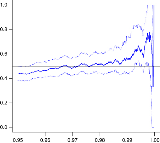
Figure 7.7 Estimator (continuous line) and confidence intervals (dotted lines) of the extremal index as a function of the quantile level  , for a sequence of high values of the threshold
  (seen as a quantile of the
  -coordinate). True value of
  close to 0.5.
Figure 7.8 presents the regenerative Bootstrap distribution (Bertail and Clémençon (2006b)) of the Hill estimator, with a choice of the optimal fraction ![]() obtained by minimizing the MSE. This leads to a CI for the tail (with a error rate of 5%) of the distribution given by
obtained by minimizing the MSE. This leads to a CI for the tail (with a error rate of 5%) of the distribution given by ![]() . This suggests that for this process, the tail may be quite heavy, since even the moment of order 3 may not exist.
. This suggests that for this process, the tail may be quite heavy, since even the moment of order 3 may not exist.

Figure 7.8 Bootstrap distribution of the pseudoregenerative Hill estimator (smoothed with a Gaussian kernel), based on  bootstrap replications. Mode around 2.8.
7.8 An Application to the CAC40
We will apply our method to the daily log return of the CAC40, from 10/07/1987 to 06/16/2014, assuming that this time series follows a Markov chain. Such hypothesis has been tested by several authors (using discretization methods) on other periods, suggesting that the usual stochastic volatility models (Black and Scholes) may not be appropriate in this case (see, for instance, McQueen and Thorley (1991), Jondeaua and Rockinger (2003), Bhat and Kuma (2010), and Cont (2001)). The log returns are plotted in Figure 7.9. Notice that the time series exhibits the same features as the SETAR-ARCH model studied before. However, we do not assume here any specific model for the underlying Markov chain. We observe a lot of regeneration blocks (1567 over 6814 observations) in a small set of optimal size close to ![]() (a minorizing constant close to
(a minorizing constant close to ![]() , yielding blocks of mean size 4.35 (Figure 7.9).
, yielding blocks of mean size 4.35 (Figure 7.9).

Figure 7.9 Log returns of the CAC40, from 10/07/1987 to 06/16/2014.
We have used two different specifications for the Markov chains, a Markov chain of order 1 and 2. The results are very similar, and we thus present only the results for a specification of a Markov chain of order 1. We distinguish between the behavior of the Markov chain for the minimum and the maximum, for which both the tail index and the extremal index may be different, leading to an asymmetric behavior between gains and losses. The following table summarizes the main results: we give the value of the estimators of the tail and extremal index as well as Bootstrap CI, respectively, for the minimum and the maximum of the time series.
| Estimators/left and right tail | Min (left tail) | Max (right tail) |
| Hill tail index estimator | 0.307 | 0.328 |
| Lower CI tail index 2.5% | 0.242 | 0.273 |
| Upper CI tail index 97.5% | 0.361 | 0.389 |
| Extremal index estimator | 0.440 | 0.562 |
| Lower CI extremal index 2.5% | 0.359 | 0.494 |
| Upper CI extremal index 97.5% | 0.520 | 0.614 |
Estimators and confidence intervals for tails and extremal indexes.
The extremal index estimators are very stable when the threshold ![]() is changed, yielding very robust estimators
is changed, yielding very robust estimators![]() We emphasize that the tail of the process is very heavy since we are close to the nonexistence of the moment of order 4. A simple test based on the Bootstrap CI allows us to accept the hypothesis that
We emphasize that the tail of the process is very heavy since we are close to the nonexistence of the moment of order 4. A simple test based on the Bootstrap CI allows us to accept the hypothesis that ![]() against
against ![]() but reject the existence of the moment of order four,
but reject the existence of the moment of order four, ![]() against
against ![]() for a type I error of
for a type I error of ![]() .
.
A striking feature of these results is seemingly some asymmetry in the times series between the minimum and the maximum log returns. In both case, the process has heavy tails with a much more heavy tail for positive log returns, but with a dynamic which creates smaller clusters of extremum values for maximum (of mean size 1.78) than for minimum (of mean size 2.27). This means that losses may be less strong than gains but may be more persistent. However, a simple test (consisting in comparing the confidence regions) yields that we do not reject the hypothesis of similar tail. This goes in the same direction as Jondeaua and Rockinger (2003) on a different period with different method, rather based on the notion of weak dependence.
7.9 Conclusion
Given the ubiquity of the Markov assumption in time series modeling and applied probability models, we review in this chapter several statistical methods, specifically tailored for the Markovian framework with a view toward the extremal behavior of such processes. Precisely, this chapter looks at statistical inference for extremal events from the renewal theory angle. We recalled that certain extremal behavior features of Harris Markov chains may be also expressed in terms of regeneration cycles, namely, data segments between consecutive regeneration times ![]() (i.e., random times at which the chain forgets its past). Working on this approach, the methodology proposed in this chapter boils down to split up the observed sample path into regeneration data blocks (or into data blocks drawn from a distribution approximating the regeneration cycle's distribution, in the general case when regeneration times cannot be observed). Then the analysis boils down to examining the sequence of maxima over the resulting data segments, as if they were i.i.d., via standard statistical methods. In order to illustrate the interest of this technique, we have concentrated on several important inference problems concerning the question of estimating the sample maximum's tail, the extremal dependence index, and the tail index. However many other parameters of interest may be investigated in the same manner. The two examples given here—ruin models in insurance and times series exhibiting threshold and/or strong conditional heteroscedasticity—clearly show the potentiality of such methods in these fields. An illustration of the estimation methods to the CAC40 shows the potential of the method for real data applications.
(i.e., random times at which the chain forgets its past). Working on this approach, the methodology proposed in this chapter boils down to split up the observed sample path into regeneration data blocks (or into data blocks drawn from a distribution approximating the regeneration cycle's distribution, in the general case when regeneration times cannot be observed). Then the analysis boils down to examining the sequence of maxima over the resulting data segments, as if they were i.i.d., via standard statistical methods. In order to illustrate the interest of this technique, we have concentrated on several important inference problems concerning the question of estimating the sample maximum's tail, the extremal dependence index, and the tail index. However many other parameters of interest may be investigated in the same manner. The two examples given here—ruin models in insurance and times series exhibiting threshold and/or strong conditional heteroscedasticity—clearly show the potentiality of such methods in these fields. An illustration of the estimation methods to the CAC40 shows the potential of the method for real data applications.
References
- Asmussen, S. Extreme value theory for queues via cycle maxima. Extremes 1998a;1(2):137–168.
- Asmussen, S. Subexponential asymptotics for stochastic processes: extremal behavior, stationary distributions and first passage probabilities. Adv Appl Probab 1998b;8(2):354–374.
- Asmussen, S. Applied Probability and Queues. New York: Springer-Verlag; 2003.
- Asmussen, S., Binswanger, K., Höjgaard, B. Rare events simulation for heavy-tailed distributions. Bernoulli 2000;6:303–322.
- Beirlant, J., Dierckx, G., Goegebeur, Y., Matthys, G. Tail index estimation and an exponential regression model. Extremes 1999;2(2):177–200.
- Bertail, P., Clémençon, S. Edgeworth expansions for suitably normalized sample mean statistics of atomic Markov chains. Probab Theory Relat Fields 2004a;130(3):388–414.
- Bertail, P., Clémençon, S. Note on the regeneration-base bootstrap for atomic Markov chains. Test 2004b;16:109–122.
- Bertail, P., Clémençon, S. Regeneration-based statistics for Harris recurrent Markov chains. In: Bertail, P., Doukhan, P., Soulier, P., editors. Probability and Statistics for Dependent Data. Volume 187 of Lecture Notes in Statistics. Springer-Verlag; 2006a. pp 3–54.
- Bertail, P., Clémençon, S. Regenerative-block bootstrap for Markov chains. Bernoulli 2006b;12(4):689–712.
- Bertail, P., Clémençon, S. Approximate regenerative block-bootstrap for Markov chains. Computational Statistics and Data Analysis 2007;52(5):2739–2756.
- Bertail, P., Clémençon, S. Sharp bounds for the tails of functionals of Markov chains; 2010. 54(3):505–515.
- Bertail, P., Clémençon, S., Tressou, J. Extreme value statistics for Markov chains via the (pseudo-)regenerative method. Extremes 2009;12:327–360.
- Bertail, P., Clémençon, S., Tressou, J. A renewal approach to Markovian U-statistics. Mathematical Methods of Statistics 2011;20:79–105.
- Bertail, P., Clémençon, S., Tressou, J. Regenerative block-bootstrap confidence intervals for the tail and extremal indexes. Electronic Journal of Statistics 2013;7:1224–1248.
- Bertail, P., Clémençon, S., Tressou, J. Bootstrapping robust statistics for Markovian data applications to regenerative R- and L-statistics. J Times Ser Anal 2015;36(3):462–480.
- Bertail, P., Haeffke, C., Politis, D., White, H. A subsampling approach to estimating the distribution of diverging statistics with applications to assessing financial market risks. Journal of Econometrics 2004;120:295–326.
- Bhat, H., Kuma, N. Markov tree options pricing. Proceedings of the 4th SIAM Conference on Mathematics for Industry; 2010.
- Bingham, N.H., Goldie, C.M., Teugels, J.L. Regular variation. Encyclopedia of Mathematics and its Applications. Cambridge: Cambridge University Press; 1987.
- Bolthausen, E. The Berry-Esseen theorem for functionals of discrete Markov chains. Z Wahrsch Verw Geb 1980;54(1):59–73.
- Clémençon, S. Moment and probability inequalities for sums of bounded additive functionals of a regular Markov chains via the Nummelin splitting technique. Statistics and Probability Letters 2001;55:227–238.
- Cont, R. Empirical properties of asset returns: stylized facts and statistical issues. Quantitative Finance 2001;1:223–236.
- Deheuvels, P., Häusler, E., Mason, D. Almost sure convergence of the Hill estimator. Math Proc Camb Philos Soc 1988;104:371–381.
- Embrechts, P., Klüppelberg, C., Mikosch, T. Modelling Extremal Events for Insurance and Finance. Applications of Mathematics. Berlin: Springer-Verlag; 1997.
- Fan, J., Yao, Q. Nonlinear Time Series - Nonparametric and Parametric Methods. New York: Springer-Verlag; 2003. 576pp.
- Ferro, C., Segers, J. Inference for clusters of extreme values. J R Stat Soc Ser B Stat Methodol 2003;65(2):545–556.
- Feuerverger, A., Hall, P. Estimating a tail exponent by modelling departure from a Pareto Distribution. Ann Stat 1999;27:760–781.
- Glynn, P., Zeevi, A. Estimating tail probabilities in queues via extremal statistics. In: McDonald, D., Turner, S., editors. Analysis of Communication Networks: Call Centres, Traffic, and Performance. Providence (RI): AMS Press; 2000. p 135–158.
- Goldie, C. Implicit renewal theory and tails of solutions of random equations. Ann Appl Probab 1991;1:126–166.
- Haiman, G., Kiki, M., Puri, M. Extremes of Markov sequences. Journal of Statistical Planning Inference 1995;45:185–201.
- Hansen, N., Jensen, A. The extremal behaviour over regenerative cycles for Markov additive processes with heavy tails. Stoch Proc Appl 2005;115:579–591.
- Hill, B. A simple approach to inference about the tail of a distribution. Ann Stat 1975;3:1163–1174.
- Hsing, T. On the extreme order statistics for a stationary sequence. Stoch Proc Appl 1988;29(1):155–169.
- Hsing, T. On tail estimation using dependent data. Ann Stat 1991;19:1547–1569.
- Hsing, T. Extremal index estimation for a weakly dependent stationary sequence. Ann Stat 1993;21(4):2043–2071.
- Jain, J., Jamison, B. Contributions to Doeblin's theory of Markov processes. Z Wahrsch Verw Geb 1967;8:19–40.
- Jondeaua, E., Rockinger, M. Testing for differences in the tails of stock-market returns. Journal of Empirical Finance 2003;10(5):559–581.
- Karlsen, H.A., Tjöstheim, D. Nonparametric estimation in null recurrent time series. Ann Stat 2001;29:372–416.
- Leadbetter, M., Rootzén, H. Extremal theory for stochastic processes. Ann Probab 1988;16:431–478.
- Loynes, R. Extreme values in uniformly mixing stochastic processes. Ann Math Stat 1965;36:993–999.
- McQueen, G., Thorley, S. Are stock returns predictable? A test using Markov chains. The Journal of Finance 1991;46:239–63.
- Malinovskii, V. On some asymptotic relations and identities for Harris recurrent Markov chains. In: Statistics and Control of Stochastic Processes (Steklov seminar, Moscow, 1984). New York: Optimization Software; 1985. p 317–336.
- Malinovskii, V. Limit theorems for Harris Markov chains I. Theory Probab Appl 1987;31:269–285.
- Malinovskii, V. Limit theorems for Harris Markov chains II. Theory Probab Appl 1989;34:252–265.
- Meyn, S., Tweedie, R. Markov Chains and Stochastic Stability. London: Springer-Verlag; 1996.
- Newell, G. Asymptotic extremes for
 -dependent random variables. Ann Math Stat 1964;35:1322–1325.
 - O'Brien, G. The maximum term of uniformly mixing stationary processes. Z Wahrsch Verw Geb 1974;30:57–63.
- O'Brien, G. Extreme values for stationary and Markov sequences. Ann Probab 1987;15:281–291.
- Resnick, S. Extreme Values, Point Processes and Regular Variation. New York: Springer-Verlag; 1987.
- Resnick, S., Stărică, C. Consistency of Hill's estimator for dependent data. J Appl Probab 1995;32:139–167.
- Revuz, D. Markov Chains. 2nd ed. Amsterdam: North-Holland; 1984.
- Robert, C,Y. Inference for the limiting cluster size distribution of extreme values. Ann Stat 2009;37(1):271–310.
- Robert, C., Segers, J., Ferro, C. A sliding blocks estimator for the extremal index. Electron J Stat 2009;3:993–1020.
- Rootzén, H. Maxima and exceedances of stationary Markov chains. Adv Appl Probab 1988;20:371–390.
- Rootzén, H. Weak convergence of the tail empirical process for dependent sequences. Stoch Proc Appl 2009;119(2):468–490.
- Smith, R. The extremal index for a Markov chain. J Appl Probab 1992;29(4):37–45.
- Thorisson, H. Coupling Stationarity and Regeneration, Probability and its Applications. New York: Springer-Verlag; 2000.
- Tjöstheim, D. Non-linear time series and Markov chains. Adv Appl Probab 1990;22:587–611.