Search in book...
Toggle Font Controls
Create new playlist

Name your new playlist

Playlist description (optional)
Sign In

Email address

Password

Forgot Password?

or

Continue with Facebook

Continue with Google
Sign Up

Full Name

Email address

Confirm Email Address

Password

or

Continue with Facebook

Continue with Google

4
Classification algorithms

4.1 Data mining algorithms for classification

This chapter is dedicated to classification algorithms. Specifically, we’ll present Decision Tree, Bayesian network, and Support Vector Machine (SVM) models. The goal of these models is the same: to classify instances of an independent dataset based on patterns identified in the training dataset. However, they work in different ways. Bayesian networks are probabilistic models which visually represent the dependencies among attributes. Decision Trees perform a type of supervised segmentation by recursively partitioning the training dataset and identifying “pure” segments in respect to the target attribute, ideally with all instances landing on the same class. SVM models are machine learning models which use nonlinear mappings for classification.

Despite their different mechanisms, these algorithms perform well in most situations. But they also differ in terms of speed and “greediness” with Decision Trees being the lightest and fastest as opposed to SVMs which typically take longer training time and are also quite demanding in terms of hardware resources. Although we’ll try to present their pros and cons later in this chapter, the choice of the algorithm to use depends on the specific situation, and it is typically a trial-and-error procedure. In this chapter, we’ll focus on the explanation of the algorithms. But remember model training is just a step of the overall classification process. This process is described in detail in Chapter 2.

4.2 An overview of Decision Trees

Decision Trees belong to the class of supervised algorithms, and they are one of the most popular classification techniques. A Decision Tree is represented in an intuitive tree format, enabling the visualization of the relationships between the predictors and the target attribute.

Decision Trees are often used for insight and for the profiling of target events/attributes due to their transparency and the explanation of the predictions that they provide. They perform a kind of “supervised segmentation”: they recursively partition (split) the overall training population into “pure” subgroups, that is, homogeneous subsets in respect to the target attribute.

The training of a Decision Tree model is a top-down, “divide-and-conquer” procedure. It starts from the initial or root node which contains the entire set of the training instances. The input (predictor) that shows the best split according to the evaluation measure is selected for branching the tree. This procedure is recursively iterated, until a stop criterion is met. Through this procedure of successive partitionings, the heterogeneous training population is split into smaller, pure, homogeneous terminal leafs (segments). The procedure is further explained in Section 4.3.

4.3 The main steps of Decision Tree algorithms

Initially, all records of the training dataset belong to the root node and obviously to one of the classes of the target attribute. In the theoretical and oversimplified example presented in Figure 4.1, the root node contains eight customers, classified into two known classes (yes/no) according to their responses in a marketing campaign.
Each Decision Tree algorithm incorporates a grow method which is an attribute selection method to assess the predictive ability of the available inputs and optimally split into subsets. For each split, the effect of all predictors on the target attribute is evaluated, and the population is partitioned based on the predictor that yields the best separation. This attribute selection is repeated for many levels until the tree is fully grown. Starting from the root node, each parent node is split into child nodes. The outcomes of the selected predictor define the child nodes of the split. The child nodes in turn become parent nodes which are further split up to the leaf nodes.
Decision Tree algorithms differ in the way they handle predictors. Some algorithms are restrained to binary splits, while others do not have this limitation. Some algorithms collapse categorical inputs with more than two outcomes in an optimal way before the split. Some discretize continuous inputs, while others dichotomize them. Hence, before step 2, a preparatory step is carried out during which all inputs are appropriately transformed before being assessed for the split.
In general, the tree growing stops when perfect separation is reached, and all instances of the leaf nodes belong to the same class. Similarly, the tree growth stops when there are no more inputs available for further splitting. Finally, the tree construction can be stopped when specific user-specified terminating criteria have been met.
The Decision Tree can be easily converted to decision rules. Specifically, rules of the following format can be extracted from the tree branches:
- IF (PREDICTOR VALUES) THEN (PREDICTION = TARGET CLASS with a specific PREDICTION CONFIDENCE).
- For example:
- IF (Tenure <= 4 years and Number of different products <= 2 and Recency of last Transaction > 20 days) THEN (PREDICTION = Churner and CONFIDENCE = 0.78)
The extracted rules are exhaustive and mutually exclusive since in the fully grown tree, each record lands into only one terminal node. Each terminal node comprises a distinct rule which associates the predictors with the target outcomes. All records landing at the same terminal node get the same prediction and the same prediction confidence (probability of prediction). The path of the successive splits from the root node to each terminal node indicates the rule conditions, the combination of input characteristics that leads to a specific outcome. In general (if no misclassification costs have been defined), the majority voting method is applied, and the dominant output class of the terminal node represents the prediction of the respective rule. The dominant class percentage designates the confidence of the prediction.

In the simple Decision Tree model of Figure 4.1, the root node is partitioned into two subsets (child nodes) according to gender. Since all women rejected the offer, the “women” node is terminal due to perfect separation and can’t be partitioned any further. Hence, the first rule has been discovered and classifies all women as nonbuyers with a respective prediction confidence of 1.0 and a purchase propensity (probability of the target class, in this case yes) of 0. On the other side of the tree, three out of the five men (60%) rejected the offer; thus, if the model had stopped at this level, the prediction would have been no purchase with a respective confidence of 3/5 = 0.6. However, there is room for improvement (we also suppose that none of our stopping criteria has been met), and the algorithm proceeds by further splitting the “men” branch of the tree into smaller subgroups and child nodes.

c4-fig-0001 — *Figure 4.1* *A simple Decision Tree model*

At this level of the tree, occupation category is the best predictor since it results the optimal separation. The parent branch is partitioned into two child nodes: blue-collar and white-collar men. The node of blue-collar men presents absolute “purity” since it only contains (100%) nonbuyers. Thus, one more rule has been identified which classifies all blue-collar men as nonbuyers with a confidence of 1.0. The percentage of buyers rises at about 67% (2/3) among white-collar men which seem to constitute the target group of the promoted service. In our fictional example, the purity of this node can be further improved if we split on SMS usage. The percentage of buyers reaches 100% among white-collar men with high SMS usage, inducing a confident rule for the identification of good prospects. The previous oversimplified example may be useful in clarifying the way that Decision Trees work, yet it cannot be considered as realistic. On the contrary, we deliberately kept it as simple as possible by presenting only faultless rules and by eliminating uncertainties due to model errors and misclassifications. In real projects, we would not even dare to split nodes with a handful of records. Moreover, the resulting terminal nodes would rarely be so homogeneous. The terminal nodes typically include records of all the outcome categories but with increased purity and decreased diversity in the distribution of the categories of the outcome, compared to the overall population. In these situations, the majority rule (dominant category) defines the prediction of each terminal node. In real-world applications, models make errors. They misclassify cases and they inevitably produce confidence values lower than 1.0. That’s why data miners should thoroughly evaluate the performance of the resulted models and assess their accuracy before deployment.

4.3.1 Handling of predictors by Decision Tree models

Decision Tree models can handle both categorical and continuous predictors. Some algorithms, including Classification and Regression Trees (CART), incorporate a binary attribute selection method and are restricted to binary splits. They always split a node in two branches. Hence, before assessing a candidate categorical outcome for a split, its outcomes are optimally collapsed in the two subsets that maximize the gain in purity.

Multiway algorithms, including C5.0/C4.5 and CHAID, split a node in as many branches as the categorical input outcomes. However, they also fine-tune this splitting, returning an optimal number of child nodes, in between the binary and the maximum. More specifically, outcomes assessed as homogeneous are merged (regrouped) into fewer categories, and the categorical split is simplified without sacrificing the gained separation.

The CHAID and C5.0/C4.5 algorithms use different approaches for splitting on continuous inputs. The C5.0/C4.5 algorithm dichotomizes continuous predictors. An optimal cut point is selected, and the continuous predictor is turned into a binary one. More specifically, the distinct values of the continuous input are evaluated as potential split points. The value, typically the midpoint between two adjacent observed values, which yields the best separation, is selected as the threshold (less than vs. greater than) for splitting. The dichotomized continuous input is then challenging the rest of predictors for the best split. This approach is shown in the Decision Tree model of Figure 4.1 when the continuous SMS usage attribute is used for the final binary split of the white-collar men node. The CHAID Decision Tree algorithm uses a different method to handle continuous predictors. It discretizes them into bins of the same size and produces ordinal attributes for splitting. Hence, the original continuous fields are converted to ordinal categorical fields with ordered outcomes.

As explained earlier, multiway tree methods can split on more than two categories at any particular level in the tree. Therefore, they tend to create wider trees which reach the target discrimination faster than binary growing methods. More specifically, categorical attributes when used at a particular level of a tree are fully “utilized,” delivering their maximum separation at a single, optimal split. On the contrary, binary splits typically lead to bushier trees with more levels. A binary split may fail to yield all the information from an input with a single split. Hence, the same attribute may be used many times at successive levels of the tree, gradually improving the purity of the child nodes.

4.3.2 Using terminating criteria to prevent trivial tree growing

As explained in 4.3, a tree may be forced to stop growing even when perfect separation has not been reached, and there are available inputs for additional splits. Specifically, a tree may be halted when certain user-specified terminating rules have been met. This approach is referred to as prepruning or forward pruning, as opposed to the postpruning procedure applied in some algorithms. The scope is common—to produce smaller, simpler, and more generalizable trees that present increased accuracy when classifying unseen cases. The pruning origin however is opposite. With postpruning, a tree is fully grown and then is trimmed to a smaller tree of comparable accuracy. Prepruning trims in advance. The tree is prevented from further growing because the maximal tree depth has been reached, the additional splits provide trivial purity improvement, or the size of the terminal nodes gets too small to support stable rules.

More specifically, the split-and-grow procedure of a tree can be terminated when one of the following terminating criteria is met:

Purity improvement: A significant predictor cannot be found, and the purity improvement gained by splitting on the available predictors is considered insignificant.
Maximal tree depth: The maximum number of allowable successive splits has been reached. Users can specify in advance the maximum tree depth, the tree levels below the root node, which determines the maximum number of times the training dataset can be recursively split.
Minimal node size: The tree is splitting into nodes of unsafely small sizes. The user-defined stopping criteria concerning the minimum size for splitting (of the parent and child nodes) has been met.

4.3.3 Tree pruning

A crucial aspect to consider in the development of Decision Tree models is their stability and their ability to capture general patterns and not patterns pertaining to anomalies of the training dataset. Overfitting is the unpleasant situation when the generated model represents the outliers and the “noise” of the training instances. In such a case, the model will most probably collapse when used on unseen data.

Prepruning is a way to deal with the pitfall of overfitting by setting relatively prudent and conservative terminating criteria. The number of the tree levels should rarely be set above 6. Additionally, the requested minimum node size should be set large enough to identify rules with acceptable support. Although the respective settings also depend on the total number of records available, it is generally recommended to keep the number of records for the terminal nodes at least above 100 and if possibly between 200 and 300. This will return rules with reasonable coverage and will eliminate the risk of modeling patterns that only apply for the specific records analyzed.

Another way to address overfitting is with tree pruning. Many Decision Tree algorithms incorporate an integrated pruning procedure which trims the tree after full growth and replace specific tree branches with internal nodes. This method is referred to as postpruning or backward pruning. The main concept behind pruning is to end up with smaller and more stable trees, with simpler structure but with improved classification accuracy on independent datasets.

The main criterion for pruning a specific branch is the number of errors. The accuracy measure known as the error rate designates the percentage of the misclassified cases. The trimming is done by comparing the compound error rate of the subtree with the estimate of its parent node. Using the training instances to validate a model leads to biased and optimistic accuracy estimates. A way to tackle this is to estimate the error rates on a holdout dataset. But this would lead to a decrease in the number of the training cases. The C5.0/C4.5 algorithm uses a method called pessimistic pruning to overcome this issue. The error rates of the subtree and the candidate leaf node are estimated on the training dataset, but the inherent bias is adjusted by adding a correction to the estimates. More specifically, the upper limits of the respective confidence intervals are used. If the accuracy estimate of the internal node is less than the one of the subtree, then the subtree is pruned.

CART on the other hand use the method of cost-complexity pruning. This method uses a prune dataset and computes a cost-complexity measure which is a function of error (misclassification) rate as well as complexity (number of terminal nodes). Large impurity and a large number of leaves correspond to a high cost-complexity measure. Subtrees are trimmed so that the highest possible decrease in the cost complexity is achieved. Hence, a large subtree with trivial purity improvement is trimmed to its parent node if the cost complexity of the pruned tree is smaller than the one of the full tree.

4.4 CART, C5.0/C4.5, and CHAID and their attribute selection measures

There are various Decision Tree algorithms. All of them have the same goal of minimizing the total purity by identifying subsegments with a dominant class. However, they use different attribute selection measures and pruning strategies. In this chapter, we’ll present the splitting criteria used by the well-established and popular CART, C5.0/C4.5, and CHAID algorithms.

The data listed in Table 4.1 will be the training dataset for a simple Decision Tree example in order to explain the different splitting criteria. The data file records the responses of 50 mobile telephony customers to a test marketing campaign (response to pilot campaign yes/no). This information defines the model’s target field. Demographical (gender, profession) and behavioral (SMS and voice usage) information is also available for the customers and will be used for predicting responses.

Table 4.1 The modeling dataset for the Decision Tree example

Customer ID	Gender	Profession	Average monthly number of SMS	Average monthly number of Voice calls	Response to pilot campaign—OUTPUT FIELD
1	Male	White collar	45	100	No
2	Male	Blue collar	32	67	No
3	Male	Blue collar	57	30	No
4	Male	Blue collar	120	150	Yes
5	Female	White collar	87	81	No
6	Male	Blue collar	98	32	No
7	Female	White collar	110	78	No
8	Female	White collar	68	90	Yes
9	Male	White collar	67	90	No
10	Male	Blue collar	23	110	No
11	Female	Blue collar	57	30	No
12	Female	White collar	125	110	Yes
13	Female	White collar	87	81	No
14	Male	Blue collar	56	56	No
15	Female	White collar	56	120	No
16	Female	White collar	90	30	Yes
17	Male	White collar	78	45	No
18	Male	Blue collar	32	87	No
19	Male	Blue collar	57	30	No
20	Male	White collar	110	100	Yes
21	Female	White collar	87	81	No
22	Male	Blue collar	34	45	No
23	Female	White collar	65	32	No
24	Male	White collar	100	90	Yes
25	Male	White collar	21	56	No
26	Male	Blue collar	65	45	No
27	Female	Blue collar	57	30	No
28	Female	Blue collar	100	105	Yes
29	Female	Blue collar	132	81	No
30	Male	Blue collar	110	97	No
31	Female	White collar	112	128	No
32	Male	White collar	100	60	Yes
33	Male	White collar	45	110	No
34	Male	Blue collar	43	67	No
35	Male	Blue collar	57	30	No
36	Female	White collar	143	140	Yes
37	Female	White collar	87	81	Yes
38	Male	Blue collar	90	45	No
39	Male	White collar	130	67	No
40	Female	White collar	98	50	Yes
41	Male	White collar	67	57	No
42	Male	Blue collar	32	55	No
43	Female	Blue collar	57	30	No
44	Male	White collar	136	60	Yes
45	Male	White collar	87	81	No
46	Male	Blue collar	67	34	No
47	Male	White collar	118	111	No
48	Female	White collar	113	78	Yes
49	Female	White collar	135	167	Yes
50	Male	Blue collar	23	34	No

4.4.1 The Gini index used by CART

The CART algorithm produces binary splits based on the Gini impurity measure. Gini is a measure of dispersion that depends on the distribution of the target classes. It ranges from 0 to 1 with larger values denoting greater impurity and a balanced distribution of the target outcomes while smaller values designate lower impurity and a dominant class within the node.

Specifically, the formula of the Gini index used by the CART algorithm is the following:

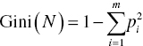
where N is the node N and p_i is the probability of target class i in node N. p_i is calculated as the proportion of cases belonging to target class i in node N. The sum is computed over the m target classes.

For example, in the case of a target field with three classes, a node with a perfectly balanced outcome distribution yields a Gini value of 0.667 (1−(3 × 0.33²)). On the contrary, a pure node with all records assigned to a single target class gets a Gini value of 0.

The Gini impurity measure of a binary split S of node N on predictor P is the weighted average of the Gini indexes of the resulting child nodes N₁ and N₂. It is calculated as follows:

where n₁ and n₂ are the number of cases of the two partitions N₁ and N₂ and n the number of cases of the parent node N.

Before each split, all predictors are optimally dichotomized as explained in 4.3.1. Categorical predictors are collapsed in those subsets that return the minimum Gini index. Analogously, for each continuous input, the best cutoff point is identified that produces the binary split with the smaller Gini index.

Then, all predictors are evaluated for the split on the basis of maximum impurity reduction or equivalently the greatest purity improvement. The purity improvement incurred by the split S of node N on predictor P is calculated as

The Gini indexes of all predictors are compared, and the attribute which yields the greater purity improvement is selected for partitioning the node N.

As an example, let’s consider the 50 cases of Table 4.1 as a root node and try to select the optimal partitioning using the Gini index. To decide the best split, the purity improvement for each possible split must be calculated and compared.

The first step is to identify the best split points for the two continuous inputs, namely, voice and SMS usage. The identified optimal cutoff values are 134 for the voice usage field and 88.5 for the SMS usage field. The two categorical inputs are binary; therefore, they are ready to participate in the split challenge.

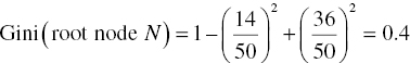
The root node contains 50 cases, 14 belonging to the target class of responders and 36 to the class of nonresponders.

The Gini index of the root node is

The profession predictor has two outcomes, white and blue collar with 28 and 22 cases each. Twelve of the white-collar and only two of the blue-collar customers responded to the campaign. Hence, the Gini index for the split on profession would be

The purity improvement incurred by splitting on profession is 0.4 − 0.0347 = 0.056.

Similarly, the Gini indexes for the rest of predictors are calculated and compared. Figure 4.2 presents the purity improvements for all possible splits and predictors as calculated by the Weight by Gini Index operator of RapidMiner.

c4-fig-0002 — *Figure 4.2* *The reduction of impurity for the four possible splits based on the Gini index*

The number of SMS field is selected for the first split as it has the minimum Gini index and returns the maximum purity improvement. The selected cutoff point of 88.5 SMS produces two child nodes which are then further split in a similar manner at subsequent levels of the CART.

The 2-level IBM SPSS Modeler CART and the respective first split on SMS usage are presented in Figure 4.3.

c4-fig-0003 — *Figure 4.3* *The first level of an IBM SPSS Modeler CART*

4.4.2 The Information Gain Ratio index used by C5.0/C4.5

The attribute selection measure used by C5.0/C4.5 is the Information Gain Ratio, an extension of the Information Gain used by their predecessor, the ID3 algorithm.

The Information Gain is based on information theory. The Information measure represents the bits needed to make out the outcome class of a particular node. It depends on the probabilities (proportions) of the outcome classes, and it can be expressed in bits which can be considered as the simple yes/no questions that are required to classify an instance. The formula for the Information or Entropy of the node N is as follows:

where N is the node N and p_i is the nonzero probability of target class i in node N. p_i is calculated as the proportion of cases belonging to target class i in node N. The measure denotes the Information required to classify the records of node N.

The Information gets its maximum value in the case of equally distributed classes and a value of zero when the number of either positive or negative cases is zero.

The Information of a split denotes the Information still needed to classify a record after partitioning on a predictor. It is calculated as the weighted average of the Information of the resulting child nodes. Specifically,

where S is the split of N on predictor P, N_j are the partitions resulted from the split which corresponds to the j outcomes of P, n_j are the instances of partition j, and n are the instances of the parent node N.

The Information gained by a split S is measured with the Information Gain index as follows:

This measure denotes the gain, the decrease in the required Information after branching the parent node N with predictor P. Before each split, all continuous predictors are optimally dichotomized as explained in 4.3.1 by identifying the ideal cutoff point for partitioning. Then, all predictors are evaluated in terms of Information reduction. The predictor which incurs the split with the maximum Information Gain is selected for the branch.

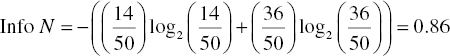
As an example, let’s consider again the 50 cases of Table 4.1 as a root node with 50 cases, 14 belonging to the target class of responders and 36 to the class of nonresponders. The cutoff values of 134 and 67.5 are selected for the number of voice and SMS calls, respectively.

The Information of the root node is

The profession binary predictor has two outcomes, white and blue collar with 28 and 22 cases respectively. Twelve of the white-collar and only two of the blue-collar customers responded to the campaign, returning an Information measure for the split on profession as follows:

The Information Gain by the split on profession is the simple difference of the above required Information values: 0.86 − 0.75 = 0.11.

Figure 4.4 presents the Information Gain measures for all inputs and partitions as calculated by the Weight by Information Gain operator of RapidMiner.

c4-fig-0004 — *Figure 4.4* *The Information gain measures for the four possible splits*

The Information Gain measure is biased toward inputs with many outcomes. It is maximal when there is one case in each partition and tends to give highly branching splits. For example, a split on an input with unique values for each training instance such as the customer ID would yield pure, single instance partitions, hence a zero Information measure for the split and maximum Information Gain.

To compensate this bias, the C5.0 and C4.5 algorithms use a normalized format of the Information Gain, the Information Gain Ratio. The Information Gain Ratio takes into account a “complexity” factor, defined by the number and the size of the resulting child nodes, and “penalizes” splits with a large number of partitions.

The Information Gain Ratio of a split is calculated by dividing the respective Information Gain by the Split Information of the input. The Split Information increases with the outcomes of the split input. The formula of the index is presented below:

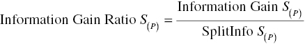
where SplitInfo S_(P) is calculated as follows:

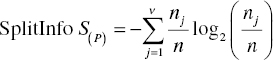
where S is the split of node N on predictor P, j the outcomes of predictor P, n_j the instances of partition j, and n the instances of the parent node.

The input with the highest Information Gain Ratio, among those with at least average Information Gain, is selected for the partition.

A simple, 2-level C5.0 tree built by IBM SPSS Modeler using the Gain Ratio split criterion is presented in Figure 4.5. The SMS usage field is used for the first partition. In the second level of the tree, heavy SMS users are further partitioned according to their profession. Note that the C5.0 algorithm uses the Information Gain criterion for selecting the optimal cutoff for continuous inputs. This explains the use of the same threshold (67.5 SMS messages) used for the relative input. Once the threshold is chosen, the selection of the best input for the split is still made on the basis of the Gain Ratio.

c4-fig-0005 — *Figure 4.5* *A simple, 2-level C5.0 Decision Tree*

4.4.3 The chi-square test used by CHAID

The CHAID algorithm uses the statistical chi-square (χ²) test of independence as the attribute selection measure.

The CHAID Decision Tree algorithm works in three main steps:

Before deciding the best split, it discretizes the continuous inputs into 10 or more bins of equal size.
Subsequently, as mentioned in 4.3.1, the categories of each input attribute, are further collapsed at an optimal number. Once again, the chi-square test of independence is applied for regrouping the input categories which are similar in respect to the target.
Finally, a series of chi-square tests are carried out to examine the null hypothesis of the independence of the binary target with each of the optimally regrouped input. The input with the strongest correlation with the target is selected for the split.

To present the basics of the chi-square test, let’s consider a two-way contingency table, a simple cross-tab of the outcomes of two categorical variables, in our case the target and an input. These two variables are considered statistically independent if the probability that an instance belongs to a certain cell is simply the product of the marginal probabilities. Hence, under the independence hypothesis:

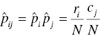
where is the probability of the cell i, j, the probability of the outcome i of the row variable, the probability of the outcome j of the column variable, N the grand total number of cases, r_i the ith row’s subtotal number of cases, and c_j the jth column’s subtotal number of cases.

Equivalently, by multiplying the two terms of the above equation with N the total number of cases, we can state our hypothesis in terms of the observed and the expected frequencies. More specifically, the two variables are independent if the expected number of cases that fall at the cell i, j of row i and column j equals to the observed number of cases in the cell:

where denotes the expected number of cases in a cell under the hypothesis of independence.

The test of independence is based on comparing the residuals which are the differences between the observed and the expected frequencies. The Pearson chi-square statistic is calculated by summing the residuals over all cells of the contingency table as follows:

where is the expected frequencies and O_ij is the observed frequencies of the cell i, j.

By using statistics, we can calculate the probability that a random sample would return a chi-square value at least as large as the one observed, if the null hypothesis of independence holds true. This probability is called the p-value or the observed significance level, and it is tested against a predetermined threshold which is called the significance level of the statistical test or α. If the p-value is small enough, hence if the probability of observing such large residuals is small, typically lower than 0.05 (5%), the null hypothesis of independence is rejected.

The CHAID algorithm evaluates for the split all the statistically significant inputs for which the hypothesis of independence is rejected. The input with the lowest p-value is selected for the split.

As an example, let’s consider once again the 50 cases of Table 4.1 as a root node and try to compare predictors in terms of the Pearson chi-square statistic. Table 4.2 presents the cross-tabulation of the target (response to pilot campaign) with the profession input and the relevant observed and expected frequencies.

Table 4.2 A cross-tab of the outcome with the profession input

Profession–response to pilot campaign—OUTPUT FIELD cross-tabulation
			Response to pilot campaign—OUTPUT FIELD		Total
			No	Yes	Total
Profession	Blue collar	Count	20.00	2.00	22.00
		Expected count	15.84	6.16	22.00
		Residual	4.16	−4.16
	White collar	Count	16.00	12.00	28.00
		Expected count	20.16	7.84	28.00
		Residual	−4.16	4.16
Total		Count	36	36.00	14.00
		Expected count	36.0	36.00	14.00

The chi-square statistic for the test of independence is calculated as follows:

The chi-square statistic of 6.97 corresponds to a p-value of 0.008. Since this value is lower than the significance level of 0.05, the independence hypothesis is rejected, and the profession input is considered a significant predictor. Hence, it’ll compete with the rest of significant predictors for partitioning the root node.

Figure 4.6 shows a comparison of the inputs in terms of the chi-square statistical test, as presented by the IBM SPSS Modeler interactive CHAID tree algorithm. The last column designates the test’s p-values for each input. The (binned) number of SMS input yields the lowest p-value value, and as shown in Figure 4.7, it is chosen for the first split.

c4-fig-0006 — *Figure 4.6* *Selecting predictors for split using the CHAID algorithm and the chi-square statistic*

c4-fig-0007 — *Figure 4.7* *A simple, 2-level CHAID Decision Tree*

@Modeling tech tips

The IBM SPSS Modeler CHAID Decision Trees

In Figures 4.8, 4.9, and 4.10 and in Table 4.3, the IBM SPSS Modeler CHAID parameters are presented and explained.

Figure 4.8 The IBM SPSS Modeler CHAID growing algorithm options

Figure 4.9 The Modeler CHAID Advanced options

Figure 4.10 The Modeler CHAID Stopping Rules

Table 4.3 The Modeler CHAID parameters

Option	Explanation/effect
Tree growing algorithm	This option determines the tree growth method. CHAID is the Modeler’s default option and the tree-growing method recommended to start with in most classification tasks
Tree growing algorithm	Worth trying alternatives: Exhaustive CHAID, a modification of the CHAID algorithm that takes longer to be trained but often gives high-quality results. Users should also try other Decision Tree algorithms and C5.0 in particular
Significance level for splitting	This option determines the significance level for the chi-square statistical test used for splitting. A split is performed only if a significant predictor can be found, that is, the p-value of the corresponding statistical test is less than the specified alpha for splitting
Significance level for splitting	In plain language, this means that by increasing the alpha for splitting value (normally up to 0.10), the test for splitting becomes less strict, and splitting is made easier, resulting in potentially larger trees. A tree previously terminated due to nonsignificant predictors may be further grown because of loosening the test’s criteria. Lower values (normally up to 0.01) tend to give smaller trees. The default value of 0.05 is adequate in most situations
Significance level for merging	This option determines the significance level for the merging of predictor categories. Higher values (normally up to 0.10) hinder the merging of predictor categories, and a value of 1.0 totally prevents merging. Lower values (normally up to 0.01) facilitate the collapsing of predictor categories. Once again, the default value of 0.05 is the most common choice
Minimum records in parent and child branch	These options specify the minimum allowable number of records in the parent and the child nodes of the tree. The tree growth stops if the size of the parent or of the resulting child nodes is less than the specified values. The size of the parent node should always be set higher (typically two times higher) than the corresponding size of the child nodes
	The requested values can be expressed in terms of percentage of overall training data or in terms of absolute number of records
	Although the respective settings also depend on the total number of records available, it is generally recommended to keep the number of records for the terminal (child) nodes at least above 50 and if possibly even higher. Large values on these settings provide robust rules “supported” by many cases/records which we expect to perform well when used in new datasets. Remember that the CHAID algorithm does not employ a postpruning method
Maximum tree depth/levels below root	This option determines the maximum allowable number of consecutive partitions of the data. Although this option is also related to the available number of records, users should try to achieve effective results without ending up with bushy and complicated trees
	For trees mainly constructed for profiling purposes, a depth of 3–4 levels is typically adequate
	For modeling purposes, a depth of 5–7 levels is sufficient, whereas larger trees, even when the available number of records allows them, would probably provide complicated rules, hard to examine and evaluate

The IBM SPSS Modeler C5.0 Decision Trees

The C5.0, the successor of the C4.5 and of the ID3 algorithm, is offered by the IBM SPSS Modeler with the parameters presented in Figure 4.11 and Table 4.4.

Figure 4.11 The Modeler C5.0 Model settings

Table 4.4 The Modeler C5.0 parameters

Option	Explanation/effect
Output type	The Decision Tree setting (recommended) is selected for building a Decision Tree with exhaustive and mutually exclusive rules which cover all the instances. The Rule set setting is used for developing decision rule sets
Group symbolics	Enables merging of predictors’ outcomes for simpler and clearer trees. It can be applied to categorical inputs. Although it is not the default setting, it is recommended since it leads to less fragmented trees
Use Boosting	A worth-trying ensemble-modeling technique, although demanding in terms of modeling time and resources. It uses the Adaptive Boosting (AdaBoost) method to build and combine a set of individual models. The first model is built the usual way, the second one focuses on the “hard” cases which were misclassified by the first one, and so on. A (confidence-weighted) voting procedure is applied to determine the final prediction and confidences
Pruning severity (Expert option)	C5.0 builds Decision Trees in two phases. A large tree is first grown which is then “pruned” by removing parts with high error rates. At the first stage of “local” pruning, each subtree is tested to decide whether it should be replaced by a leaf node or a subbranch. Then, a second, global pruning stage assesses the performance of the tree as a whole for further pruning. The pruning severity option affects the first stage of pruning. It corresponds to (1—the confidence level) used for the pessimistic error calculation of pruning, and hence it affects the way that error rates are estimated and the severity of pruning
Pruning severity (Expert option)	The higher the value, the more severe the first stage pruning. The default value of 75% corresponds to a confidence value of 25%, and it is suitable for most purposes. A higher value could be tested for more drastic pruning
Winnow attributes (Expert option)	This option applies an integrated feature selection procedure for prepruning. Irrelevant predictors are identified and omitted from the model training. This option might be proved useful when there are a large number of inputs
Use global pruning (Expert option)	This option toggles on/off the second phase of global pruning. Global pruning is recommended for most Decision Tree models. Turning off global pruning can be tried especially when developing rule sets
Minimum records per child branch (Expert option)	A branch will be spit only if two or more of the resulting subbranches have at least this number of records. Values around 50 are a reasonable starting point, especially in cases with many noisy data. In any case, leaf nodes with a trivial number of instances should be avoided for stability reasons

The IBM SPSS Modeler CART

The main parameters of the IBM SPSS Modeler CART algorithm are summarized in Figures 4.12, 4.13, and 4.14 and Table 4.5.

Figure 4.12 The Modeler CART Basics options

Figure 4.13 The Modeler CART Advanced options

Figure 4.14 The Modeler CART Stopping criteria

Table 4.5 The Modeler CART parameters

Option	Explanation/effect
Impurity measure for categorical targets	This setting is available in the Expert tab, and users can select the impurity measure and hence the attribute selection method for the tree among Gini, Twoing, and Ordered. The Gini index presented in 4.4.1 is the recommended option
Prune tree (maximum difference in risk in standard errors)	The prune tree option employs cost-complexity pruning; it is turned on and should be normally kept on to produce trimmed, generalizable trees which are not memorizing the noise of the training data
	Initially, the tree is fully grown according to the specified stopping criteria before trimmed. The cost-complexity pruning method removes a tree branch if the cost associated with having a more complex tree exceeds the gain associated with having another branch. It uses an index that measures both the risk estimate (misclassification rate) and the complexity, the number of terminal nodes of the tree
	The standard error rule compares the pruned trees with the fully grown tree in terms of their risk estimates. The multiplier of the standard error rule defines the boundary of the acceptable risk estimate. Thus, a multiplier of one will yield the smallest tree whose risk estimate is up to (1 × standard error) larger than that of the full tree. Lower values of the multiplier would produce larger, slightly trimmed trees
Minimum change in impurity	A prepruning option which specifies the minimum acceptable purity improvement in order to create a new split. A split will be done only if the purity improvement is at least as large as the specified value. Hence, by lowering the minimum acceptable value, we allow more splits and larger trees
Minimum records in parent and child branch	These options specify the minimum allowable number of records in the parent and child nodes of the tree. The tree growth stops if the size of the parent or of the resulting child nodes is less than the specified values. The size of the parent node should always be set higher (typically two times higher) than the corresponding size of the child nodes
	The requested values can be expressed in terms of percentage of overall training data or in terms of absolute number of records
	Since CART employs a postpruning method, the number of records of the terminal nodes should not be set as high as in CHAID trees. Values around 50 are usually a good starting point for trial and error
Maximum tree depth/levels below root	As in CHAID, this option specifies the maximum allowable number of consecutive partitions of the data. Given that the fully grown tree will be finally trimmed, a larger number of levels than in CHAID are selected, typically 6+
Overfit prevention set (%)	Specifies the portion of the dataset used to track errors during model training in order to prevent overfitting. The default value is 30%

The RapidMiner Decision Trees

The RapidMiner Decision Tree algorithm works similar with the C4.5 and CART algorithms. It applies recursive partitioning with successive splits based on the Gini, the Information Gain, or the Information Gain Ratio measures. The algorithm also employs prepruning as well as prostpruning techniques to avoid overspecific and overfitted models.

The relevant parameters are shown in Figure 4.15 and discussed in Table 4.6.

Figure 4.15 The RapidMiner Decision Tree options

Table 4.6 The RapidMiner Decision Tree parameters

Option	Explanation/effect
Criterion	This option determines the attribute selection method used for producing the tree. The available grow methods include the Information Gain and the Information Gain Ratio presented in 4.4.2 and the Gini index presented in 4.4.1. The Information Gain Ratio is the default option; the other two methods are certainly worth trying
Minimal size for split/minimal leaf size	The next four options—minimal size for split, minimal leaf size, minimal gain, and maximal depth—are related with the prepruning and define the terminating criteria of the model. The tree is prevented from growing if the sizes of the parent or terminal nodes are lower than the respective thresholds. Large enough threshold values should be set in order to identify rules with adequate support
Maximal depth	The maximum allowable number of consecutive splits. Although the produced tree is finally trimmed, you’ll typically have to decrease the number of levels from the default (20) to values between 6 and 10
Minimal gain	The minimum acceptable purity improvement in order to branch a node. Lower values correspond to less stringent split criteria and lead to larger trees. The default threshold of 0.1 is quite strict in many situations, and you may have to try lower values
Confidence	The confidence level used for the pessimistic error rate calculation of pruning. Although the default value works well in most situations, it can be tweaked to control the severity of pruning. Smaller values than the default (25%) allow heavier pruning and produce smaller trees, while larger values result in less pruning
No prepruning/no pruning	By default, prepruning and postpruning are applied, and normally, this is the recommended approach for model training. However, analysts can disable these options by selecting the relevant checkboxes

Microsoft Decision Trees

Decision Tree models are also available in Data Mining for Excel. The classification algorithm and the settings for fine-tuning are set through the Algorithm Parameters menu of the Classify Wizard as seen in Figure 4.16 and discussed in Table 4.7.

Figure 4.16 The Microsoft Decision Tree parameters

Microsoft Decision Trees is a recursive partitioning algorithm. The attribute selection methods used to determine the splits include measures based on Entropy (the Information measure presented in 4.4.2) and Bayesian networks.

The algorithm incorporates a preprocessing feature selection step to screen inputs and focus on the most useful predictors. In terms of inputs’ handling, continuous predictors are optimally discretized for the needs of classification models. Initially, the continuous inputs are binned into chunks of equal range. Then, the bins are optimally regrouped based on the selected split measure in order to yield an optimized split score. Finally, the input with the best score is selected for branching.

The same approach of optimal regrouping is also the default approach for categorical inputs.

Table 4.7 The Microsoft Decision Trees parameters

Option	Explanation/effect
Complexity penalty	A parameter related with prepruning which controls the growth of the Decision Tree. Its values range from 0 to 1. Lower values increase the allowable number of splits, producing bushier trees. On the contrary, higher values, close to 1, penalize the tree growth, resulting smaller trees. The default value is based on the number of inputs as follows:
	For 1 through 9 predictors, the default value of 0.5 is applied
	For 10 through 99 predictors, the default value of 0.9 is applied
	For 100+ predictors, the default value of 0.99 is applied.
Maximum input attributes	A threshold parameter for the integrated feature selection. Feature selection is invoked if the number of inputs is greater than the specified value. A value of 0 turns off feature selection (the MAXIMUM OUTPUT ATTRIBUTES option is relevant only for regression tree models)
Minimum support	This parameter is a terminating criterion related with prepruning, and it defines the acceptable leaf size. More specifically, it determines the minimum support which is the minimum number of cases in a leaf node (as a percentage of the total cases or as absolute frequency) in order for a split to be allowed
Score method	The available attribute selection methods include the Information measure based on Entropy and two measures based on Bayesian networks: the Bayesian with K2 prior and the Bayesian Dirichlet Equivalent (BDE) with Uniform prior (the default), all of which are scalable and worth trying
Split method	Determines the handling of predictors for split. SPLIT METHOD = 1 produces binary splits. SPLIT METHOD = 2 is used for multiway splits with a branch for each outcome of the predictor. The default and recommended SPLIT METHOD = 3 is a hybrid method, which combines the previous two methods for optimal regrouping of predictors to yield the best split

4.5 Bayesian networks

Naïve Bayesian networks are statistical models based on the Bayes theorem. They are probabilistic models as they estimate the probabilities of belonging to each target class. In fact, their classification is based on comparing the estimated target class probabilities, given the information provided by the inputs.

In spite their simplicity and their naïve assumption of independence, Naïve Bayesian classifiers have shown remarkable performance in many situations comparable to more “sophisticated” classifiers. However, this is not always the case. Bayesian belief networks are an advancement of the Naïve Bayes algorithm. The dependence restrictions of Naïve Bayes are relaxed, achieving improved classification accuracy. Additionally, they are graphical models, providing a visual representation of the relationships between the variables.

4.6 Naïve Bayesian networks

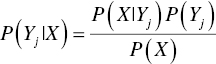
The Bayes rule of conditional probability, named after the clergyman Thomas Bayes, states that if we have a hypothesis H and evidence E, then

In classification problems, our hypothesis is the membership to a target class. We want to estimate the corresponding probabilities, given the evidence, the particular combination of input values. Hence, assuming n inputs X_i and m target classes Y_j, for an instance with input values X = (x₁, x₂, …, x_n), the probability of belonging to the target class Y_j is

or equivalently

P(H) or P(Y_j) is the prior probability of the target class (of the hypothesis), and it is independent of the values of the inputs X. P(Y_j|X) is the posterior probability of the hypothesis given the evidence. It is the probability of the target class conditioned on the observed values of the predictors.

An instance is classified to the target class with the maximum posterior probability. Hence, we need to estimate and compare the probabilities of P(Y_j|X) for each target class Y_j. We need to maximize the P(Y_j|X) and label the instance with the class which returns the maximum conditional probability. Therefore, we don’t need to worry about the probability of evidence. As it is the common denominator for all target classes, it can be ignored. However, in a final step, the estimated probabilities must be normalized by dividing with their sum so that they add to 1.

The prior probability P(Y_j) can be easily calculated as the percentage of the target class j in the training dataset.

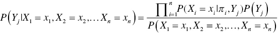
So that leaves us with the calculation of P(X|Y_j). To simplify calculations, in the Naïve Bayesian models, we “naïvely” assume class conditional independence. More specifically, we assume that the inputs are independent, given the target.

Having assumed independent events, we can multiply their probabilities, and the aforementioned equation of the conditional probability can be stated as follows:

The probabilities of the nominator can be easily computed for each training instance. If X_i is a categorical input, is simply the percentage of cases with the value for the input within the target class .

But what if the input is continuous? A common approach, which is also employed in IBM SPSS Modeler and Data Mining for Excel, is discretization. The continuous attribute is binned into an ordinal predictor, and the conditional probabilities are estimated for each bin based on the relevant distributions. Alternatively, a normal distribution can be assumed for the continuous input, and the probability density function can be used to estimate the respective probabilities.

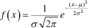
The probability density function of a continuous random variable with the normal distribution, mean μ and standard deviation σ, is a function that describes the relative likelihood for this random variable to take on a given value , and it is estimated as follows:

So, under the normal distribution assumption, in order to estimate the conditional probabilities , we only need to calculate the mean and the standard deviation of the input X_i for each target class Y_j. By plugging these two values (respectively, , ) in the above equation, the estimation of through is straightforward for any observed value of the input for the cases of the target class .

Since the estimation is based on the multiplication of conditional probabilities, things get messy if we end up with a conditional probability of 0. This occurs when we have no cases for a particular combination of input–output values. In such situations, a single 0 leads to an overall equal to 0. A common approach to override this problem is to add 1 or a small constant to each count. This adjustment, known as the Laplace correction, ensures that possible zero counts would not distort our estimation.

In the final step of the algorithm, for each training (or scoring) instance, the conditional probabilities , which as explained are analogous to , are assessed for each target class j. The instance is classified to the target class with the maximum probability.

Figure 4.17 shows a RapidMiner process with a Naïve Bayes operator used for developing a classification model.

c4-fig-0017 — *Figure 4.17* *A RapidMiner process for training a Naïve Bayes classification model*

As Naïve Bayes is a probabilistic algorithm, it provides estimates of the probabilities (prediction confidences) of the output classes as shown in Figure 4.18. The probabilities are estimated when the data pass through the Apply Model operator which is used for model scoring.

c4-fig-0018 — *Figure 4.18* *The prediction and probabilities estimated from a RapidMiner Naïve Bayes classification model*

Data Mining for Excel also supports the Naïve Bayes algorithm. As stated in the Classify Wizard menu (Figure 4.19), the Naïve Bayes algorithm assumes independence of the inputs, given the output. It also requires discretized inputs. Continuous inputs can be discretized into a specified number of equal-width buckets using the Explore wizard.

c4-fig-0019 — *Figure 4.19* *The Microsoft Naïve Bayes algorithm in the Classify Wizard of Data Mining for Excel*

The Dependency network included in the model’s results illustrates the inputs–output relationships as shown in Figure 4.20.

c4-fig-0020 — *Figure 4.20* *The Microsoft Naïve Bayes Dependency network in Data Mining for Excel*

The Attribute Profiles output presented in Figure 4.21 depicts the percentages of the input categories, which are named as “states” in Data Mining for Excel, within each target class (in this example, response to pilot campaign: Yes/No). In other words, it illustrates the conditional probabilities discussed earlier.

c4-fig-0021 — *Figure 4.21* *The Data Mining for Excel Attribute Profiles report presents the conditional probabilities used by the Naïve Bayes algorithm*

The Attribute Characteristics shown in Figure 4.22 sorts the input categories in descending order of their conditional probabilities (given the selected target class). In other words, it depicts the conditional probabilities discussed earlier.

c4-fig-0022 — *Figure 4.22* *The Data Mining for Excel Attribute Characteristics report sorts the input categories according to their conditional probabilities for the selected target class*

Like the Decision Tree models presented previously, the Naïve Bayes results indicate that the response to the pilot campaign is more likely among white-collar professionals, heavy SMS users, and women.

4.7 Bayesian belief networks

Bayesian belief networks are an improvement over Naïve Bayes models. The class conditional independence, assumed by the Naïve Bayes algorithm, is relaxed. Instead of assuming independence between the inputs, we allow dependencies between subsets of variables. In Naïve Bayes, each input only depends on the target variable. In Bayesian belief networks, however, a subset of “parent” variables is identified for each variable. Our assumption now is less strict since each variable is assumed to be independent of other variables given its parents.

Bayesian belief networks are graphical, probabilistic models, represented by acyclic graphs. Each variable, including the output, is represented by a node in the graph. The nodes are connected by directed edges, in a way that they are no cycles (directed acyclic graph). The connecting arcs of the graph point from the parent to the child node, depicting conditional probabilities. Hence, each belief network consists of a graph and the conditional probability table (CPT) with the conditional probabilities for each node. The Naïve Bayes network is a simple belief network with an arc leading from the output node to each input attribute.

Similarly with Naïve Bayes models, the goal is to estimate the target class probabilities. As in 4.6, assuming n inputs X_i and m target classes Y_j, for an instance with input values X = (x₁, x₂, …, x_n), the posterior probabilities P(Y_j|X), given the evidence, are calculated as follows:

or equivalently

Since each variable is conditionally independent of its nondescendants in the graph given its parents, the above formula becomes

where is the parent set of the input , besides Y.

Similarly with Naïve Bayes, an instance is classified to the target class which maximizes the posterior probability P(Y_j|X). The probability of the denominator can be ignored, and the estimated probabilities are normalized to sum to 1.

In the Tree Augmented Naïve Bayes models (TAN Bayesian models), a class of belief networks, we allow each predictor to depend on another predictor, in addition to the output. The network has the structure shown in Figure 4.23.

c4-fig-0023 — *Figure 4.23* *The structure of Tree Augmented Naïve Bayes models (TAN Bayesian models)*

A CPT is associated with each input node of the network denoting the conditional probabilities . Each column of the CPT corresponds to a category value of the input (Figure 4.26). Note that the continuous inputs are discretized. Each row of the table corresponds to a target class–parent input value combination. Hence, the CPT summarizes the conditional probabilities for each value of the input across all combinations of the values of its parents.

An instance is defined by its input values . To classify the instance, we have to look up the CPT entries which correspond to its observed values. Then, we simply multiply the respective entries. This procedure is repeated for each target class, and the instance is classified to the class which yields the maximum conditional probability.

A TAN network trained in IBM SPSS Modeler is shown in Figure 4.24.

c4-fig-0024 — *Figure 4.24* *A TAN Bayesian network built in IBM SPSS Modeler*

The network is consisted of five nodes, one for the output (response to pilot campaign field) and one for each input. Directed arcs connect each parent with its descendants. Each input node has the output as its parent. Furthermore, the Gender node is the second parent for the other inputs: Profession, Average monthly number of Voice calls, and Average monthly number of SMS fields.

Besides its topology, the network is defined by the CPT which explain each node. The CPT of the example are depicted in Figures 4.25, 4.26, 4.27, 4.28, and 4.29. Note that the continuous inputs have been automatically discretized in five bins of equal width.

c4-fig-0025 — *Figure 4.25* *The probabilities of the output (response to pilot campaign)*

c4-fig-0026 — *Figure 4.26* *The conditional probabilities of the profession input attribute*

c4-fig-0027 — *Figure 4.27* *The conditional probabilities of the voice calls input attribute*

c4-fig-0028 — *Figure 4.28* *The conditional probabilities of the SMS calls input attribute*

c4-fig-0029 — *Figure 4.29* *The conditional probabilities of the gender input attribute*

Now, let’s consider a case with the following characteristics: Gender = Female, Profession = White collar, Average monthly number of SMS = 87, and Average monthly number of Voice calls = 81. This case is in row 5 of the training dataset shown in Figure 4.30.

c4-fig-0030 — *Figure 4.30* *The training dataset of the TAN Bayesian network*

In order to classify this instance, the relevant CPT entries have to be examined.

The conditional probability of Response = Yes given the evidence is calculated as follows:

P(Response = Yes | Gender = Female, Profession = White collar, Average monthly number of SMS = 87, Average monthly number of Voice calls = 81) ~ (is analogous to)
P(Gender = Female | Response = Yes)*
P(Profession = White collar | Response = Yes, Gender = Female)*
P(Average monthly number of SMS in [74, 97] | Response = Yes, Gender = Female)*
P(Average monthly number of Voice calls in [72.8, 95.2] | Response = Yes, Gender = Female)*
P(Response = Yes) = 0.63 * 0.87 * 0.22 * 0.33 * 0.29 = 0.011

The conditional probability of Response = No, for the same case, given the evidence is calculated as follows:

P(Response = No | Gender = Female, Profession = White collar, Average monthly number of SMS = 87, Average monthly number of Voice calls = 81) ~
P(Gender = Female | Response = No)*
P(Profession = White collar | Response = No, Gender = Female)*
P(Average monthly number of SMS in [74, 97] | Response = No, Gender = Female)*
P(Average monthly number of Voice calls in [72.8, 95.2] | Response = No, Gender = Female)*
P(Response = No) = 0.31 * 0.63 * 0.27 * 0.44 * 0.71 = 0.016

Finally, the case is classified as nonresponder since the no conditional probability is higher. The probability of no is normalized to 0.016 / (0.011 + 0.016) = 0.59. The probability of yes is simply (1 − 0.59) or 0.41.

As shown in Figure 4.30, the predicted class for the scored instance is denoted in the field named $B-Response, along with its confidence, listed in the field named $BP-Response. The estimated probabilities for each target class are listed in the fields named as $BP-no and $BP-YES. The probability of no is equal to the prediction confidence.

@Modeling tech tips

The IBM SPSS Modeler 00392ayesian networks

Bayesian belief networks are available in IBM SPSS Modeler. The main parameters of the algorithm are presented in Figures 4.31 and 4.32 and in Table 4.8.

Figure 4.31 The IBM SPSS Modeler Bayesian networks model options

Figure 4.32 The IBM SPSS Modeler Bayesian networks model Expert options

Table 4.8 The Modeler Bayesian networks parameters

Option	Explanation/effect
Structure type	This option determines the network’s structure type. The TAN option builds a Tree Augmented Naïve Bayes model (TAN Bayesian models), a more complex but more efficient alternative over Naïve Bayes. The Markov Blanket estimation has even less assumptions regarding the variables’ dependencies. It identifies all the variables in the network that are needed to predict the output. As it produces more complex networks, it is more demanding in terms of processing times and resources
Include feature selection preprocessing step	Invokes a feature selection preprocessing step to identify and filter out the inputs with marginal predictive ability. Especially useful in the case of large datasets with many inputs
Paremeter learning method	The Maximum Likelihood estimation is the default option for parameter learning. The “Bayes adjustment” option is a useful alternative, especially in the case of small datasets. It applies an adjustment to overcome possible zero counts in the input–output value combinations
Append all probabilities	Bayesian networks are probabilistic models that can estimate the probabilities of belonging to each target class. This option, available in the Expert options tab, calculates the relevant fields
Independence test	Determines the test to be applied to identify the independencies among variables. The Likelihood ratio (the default option) or the chi-square test is used to find the relationships among variables and build the network
	The Independence test options are only available if you select either the feature selection preprocessing step or a Structure type of Markov Blanket on the Model tab
	The significance level option sets the threshold value for the independence tests. The lower the value, the more strict the feature selection test and less inputs are retained. Similarly, lower values yield simpler network structures with fewer connecting arcs in the network; the default level is 0.01
	The feature selection process can be further tweaked by selecting the “Maximum number of retained inputs” as well as a set of inputs which are “Always selected”

Microsoft Naïve Bayes

The Naïve Bayes classifiers are also offered by Data Mining for Excel. The model is built through the Classify Wizard. The algorithm parameters are presented in Figure 4.33 and discussed in Table 4.9.

Figure 4.33 The Microsoft Naïve Bayes parameters

Table 4.9 The Microsoft Naïve Bayes parameters

Option	Explanation/effect
Maximum input attributes	A threshold parameter for the integrated feature selection preprocessing step. Feature selection is invoked if the number of inputs is greater than the specified value
	A value of 0 turns off feature selection
	The default value is 255
Maximum states	This option determines the maximum number of input categories (“states”) that the algorithm will analyze. If an attribute has more categories than the specified threshold, then only the most frequent categories will be used, and the remaining and rare categories are treated as missing
	The default value is 100
Minimum dependency probability	It sets a minimum threshold probability value for the independence tests between the inputs and the outputs. This parameter does not affect the model training or prediction, but it limits the size of the output content returned by the algorithm. Increasing the value reduces the number of inputs in the network
Minimum dependency probability	It ranges from 0 to 1; the default level is 0.1

The RapidMiner Naïve Bayes

The RapidMiner Naïve Bayes classifier is applied through the Naïve Bayes operator. A “Laplace correction” option is available to reduce the impact of zero counts in the estimation of the conditional probabilities.

4.8 Support vector machines

SVMs work by mapping the inputs to a transformed input space of a higher dimension. The original inputs are appropriately transformed through nonlinear functions. The selection of the appropriate nonlinear mapping is a trial-and-error procedure in which different transformation functions are tested in turn and compared.

Once the inputs are mapped into a richer feature space, SVMs search for the optimal, linear decision class boundary that best separates the target classes. In the simple case of two inputs, the decision boundary is a simple straight line. In the general case of n inputs, it is a hyperplane.

Overall SVMs are highly accurate classifiers as they can capture and model nonlinear data patterns and relationships. On the other hand, they are also highly demanding in terms of processing resources and training time.

4.8.1 Linearly separable data

In this paragraph, we’ll try to explain what does an “optimal” decision boundary means. Initially, we assume that the data are linearly separable, meaning that there exists a linear decision boundary that separates the positive from the negative instances.

A linear classifier is based on a linear discriminant function of the form

where X denotes the vector of the inputs x_i, w denotes the vector of weights, and b can be considered an additional weight (w0). Hence, the discriminant function is the dot product of the inputs’ vector with the vector of weights w, which, along with b, are estimated by the algorithm.¹

A separating hyperplane can be written as

The hyperplane separates the space into two regions. The decision boundary is defined by the hyperplane. The sign of the discriminant function f(X) denotes on which side of the hyperplane a case falls and hence on which class is classified.

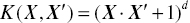
For illustrative purposes, let’s consider a classification problem with two inputs x₁ and x₂. In such cases, the decision boundary is a simple straight line. Because we have assumed that the data are linearly separable, no mapping to higher input dimensions is required. In the next paragraph, we’ll generalize the SVM approach to situations where the data are linearly inseparable.

The separating hyperplane for the simple case of two inputs is a straight line:

Cases for which lie above the separating line, while cases for which lie below. The instances are classified based on which side of the hyperplane they land.

As shown in Figure 4.34, there are an infinite number of lines that can provide complete separation in the feature space of the inputs.

c4-fig-0034 — *Figure 4.34* *A set of separating lines in the input feature space, in the case of linearly separable data*

The SVM approach is to identify the maximum marginal hyperplane (MMH). It seeks for the optimal separating hyperplane between the two classes by maximizing the margin between the classes’ closest points. The points that lie on the margins are known as the support vectors, and the middle of the margin is the optimal separating hyperplane.

In Figure 4.35, a separating line is shown. It completely separates the positive cases, depicted as transparent dots, from the negative ones which are depicted as solid dots. The marked data points correspond to the support vectors since they are the instances which are closest to the decision boundary. They define the margin with which the two classes are separated. The MMH is the straight line in the middle of the margin. The support vectors are the hardest cases to be classified as they are equally close to the MMH.

c4-fig-0035 — *Figure 4.35* *A separating hyperplane with the support vectors and the margin in a classification problem with two inputs and linear data*

In Figure 4.36, a different separating line is shown. This line also provides complete separation between the target classes. So which one is the optimal and should be selected for classifying new cases?

c4-fig-0036 — *Figure 4.36* *An alternative separating hyperplane with its support vectors and its margin for the same linear data*

As explained earlier, SVMs seek for large margin classifiers. Hence, the MMH depicted in Figure 4.35 is preferred to the one shown in Figure 4.36. Due to its larger margin, we expect it to be more accurate in classifying unseen cases. A wider margin indicates a generalizable classifier, not inclined to overfitting.

In practice, a greater margin is achieved on the cost of sacrificing accuracy. A small amount of misclassification can be accepted in order to widen the margin and favor general classifiers. On the other hand, the margin can also be narrowed a little to increase the accuracy. The SVM algorithms incorporate a regularization parameter C which sets the relative importance of maximizing the margin. It balances the trade-off between the margin and the accuracy. Typically, experimentation is needed with different values of this parameter to yield the optimal classifier.

The training of an SVM model and the search for the MMH and its support vectors are a quadratic optimization problem. Once the classifier is trained, it can be used to classify new cases. Cases with null values at one or more inputs are not scored.

4.8.2 Linearly inseparable data

Let’s consider again a classification problem with two predictors, x₁, x₂. Only in this case let’s consider linearly inseparable data. Therefore, no straight line can be drawn in the plane defined by x₁, x₂ that could adequately separate the cases of the target classes. In such cases, a nonlinear mapping of the original inputs can be applied. This mapping shifts the dimensions of the input space in such a way that an optimal, linear separating hyperplane can then be found. The cases are projected into a (usually) higher-dimensional space where they become linearly separable.

For example, in the simple case of two inputs, a Polynomial transformation ϕ: R² → R³ is

It maps the initial two inputs into three. Once the data are transformed, the algorithm searches for the optimal linear decision class boundary in the new feature space.

The decision class boundary in the new space is defined by

where is the mapping applied to the original inputs.

In the example of the simple Polynomial transformation, it can be written as

Hence, the decision boundary is linear in the new space but corresponds to an ellipse in the original space.

However, the above approach does not scale well with wide datasets and a large number of inputs. This problem is solved with the application of kernel functions. Kernel functions are used to make (implicit) nonlinear feature mapping. The training of SVM models involves the calculation of dot products between the vectors of instances. In the new feature space, this would be translated as dot products of the form

where ϕ denotes the selected mapping function.

But these calculations are computationally expensive and time consuming. But if there was a function K such that , then we wouldn’t need to make the ϕ mapping at all. Fortunately, certain functions named the kernel functions can achieve this. So, instead of mapping the inputs with ϕ and computing their dot products in the new space, we can apply a kernel function to the original inputs.

The dot product is replaced by a nonlinear kernel function. In this way, all calculations are made in the original input space, which is desirable since it is typically of much lower dimensionality. The decision boundary in the high-dimensional new feature set is identified. However, due to kernel functions, the ϕ mapping is never explicitly applied.

Two commonly used Kernel functions are:

Polynomial (of degree d): where d is a tunable parameter
(Gaussian) Radial Basis Function (RBF):
Sigmoid (or neural):

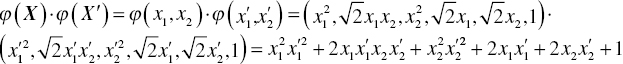
For example, the Polynomial, degree 2 kernel (quadratic kernel) for the case of two inputs would be:

The above is equal to the dot product of two instances in the feature space defined by the following transformation ϕ: R² → R⁶:

@Modeling tech tips

The IBM SPSS Modeler SVM model

Figure 4.37 and Table 4.10 present the parameters of the IBM SPSS Modeler SVM classifier.

Figure 4.37 The IBM SPSS Modeler SVM settings

The RapidMiner SVM models

RapidMiner includes several SVM models. The SVM classifier, available through the modeling operator of the same name, supports the RBF, the Polynomial, and the Sigmoid kernel functions. Its parameters are presented in Figure 4.38 (for the RBF kernel function). Since the role and the significance of SVM parameters are already explained in Table 4.10, Table 4.11 briefly presents the RapidMiner parameters.

Figure 4.38 The RapidMiner RBF Support Vector Machine model options

Table 4.11 The RapidMiner SVM parameters

Option	Explanation/effect
Convergence epsilon	Determines when the optimization algorithm converges and stops. Default value is 1.0E−1. Smaller values increase the accuracy of the model but at a cost of increased training time
C	The regularization parameter C
Kernel type	It determines the kernel function to be applied. Available kernels include radial (Radial Basis Function), Polynomial, and neural (Sigmoid)
Kernel gamma	Available when the radial (RBF) kernel function is selected. It corresponds to the parameter of the kernel function. The default value is 2
Kernel degree	The kernel degree parameter is enabled when the Polynomial kernel function is selected. It sets the Polynomial degree, the d parameter of the kernel function
Kernel a	The γ adjustable parameter for the Sigmoid (neural) kernel
Kernel b	The b (bias) parameter of the neural kernel

Overall, the fine-tuning of the SVM parameters is a trial-and-error process. The RBF kernel function is a usual initial kernel choice. However, different values of the C and γ should be tested with validation or grid search in order to select the optimal parameter values.

4.9 Summary

In this chapter, we presented three of the most accurate and powerful classification algorithms: Decision Trees, SVMs, and Bayesian networks.

SVMs are highly accurate classifiers. However, they suffer in terms of speed and transparency. They are demanding in terms of processing resources and time. This hinders their application in real business problems, especially in the case of “long” datasets with a large number of training instances. Apart from their speed problem, SVMs also lack transparency. They belong to the class of opaque classifiers whose results do not provide insight on the target event.

This is not the case with the Bayesian networks. Especially the class of Bayesian belief networks, with their graphical results, provides a comprehensive visual representation of the results and of the underlying relationships among attributes. Although faster than SVMs, the Bayesian networks in most cases are not as accurate.

Decision Trees on the other hand seem to efficiently combine accuracy, speed, and transparency. They generate simple, straightforward, and understandable rules which provide insight in the way that predictors are associated with the output. They are fast and scalable, and they can efficiently handle a large number of records and predictors.

Note

..................Content has been hidden....................

You can't read the all page of ebook, please click here login for view all page.

Option	Explanation/effect
Stopping criteria	Determines when the optimization algorithm converges and stops. Values range from 1.0E−1 to 1.0E−6. The default value of 1.0E–3 is appropriate for most classification tasks; smaller values increase the accuracy of the model but at a cost of increased training time
Regularization parameter (C)	The regularization parameter C which balances the trade-off between generalization (wider margin) and accuracy. Default value is 10. Smaller values correspond to “wider” margins, and larger values produce “broader” ones. Thus, increasing the value improves the model accuracy but with a risk of overfitting
Kernel type	It determines the kernel function to be applied. Available kernels include Radial Basis Function (RBF), Polynomial, Sigmoid, and Linear. The default function is RBF which is a reasonable first choice
RBF gamma	Available only when RBF kernel function is selected. It corresponds to the parameter of the kernel function. As a rule of thumb, values between 3/k and 6/k, where k is the number of predictors in the model, should be set as initial values. Increased values lead to improved accuracy but may also lead to overfitting
Degree	The kernel degree parameter is enabled when the Polynomial kernel function is selected. It sets the Polynomial degree, the d parameter of the kernel function. It determines the complexity of the mapping and hence of the model training time. The selected values should rarely exceed 10
Gamma	The γ adjustable parameter for the Polynomial and the Sigmoid kernels. The default value is 1. Increased values improve the mode accuracy with a risk of overfitting
Bias	Enabled only when the Polynomial or the Sigmoid kernel is selected. It corresponds to the b parameter. (Note that in IBM SPSS Modeler, the Polynomial kernel function is defined as ) The default value of 0 is appropriate in most situations

Table of Contents for 4 Classification algorithms

Create new playlist

Sign In

Sign Up

4.1 Data mining algorithms for classification

4.2 An overview of Decision Trees

4.3 The main steps of Decision Tree algorithms

4.3.1 Handling of predictors by Decision Tree models

4.3.2 Using terminating criteria to prevent trivial tree growing

4.3.3 Tree pruning

4.4 CART, C5.0/C4.5, and CHAID and their attribute selection measures

4.4.1 The Gini index used by CART

4.4.2 The Information Gain Ratio index used by C5.0/C4.5

4.4.3 The chi-square test used by CHAID

4.5 Bayesian networks

4.6 Naïve Bayesian networks

4.7 Bayesian belief networks

4.8 Support vector machines

4.8.1 Linearly separable data

4.8.2 Linearly inseparable data

4.9 Summary

Note

Table of Contents for
4 Classification algorithms