
5
Pulse Modulation
Telecommunication systems aim to provide a faithful replica of transmitted signals to be successfully decoded by distant receivers. Transmitted signals may carry analog or digital information. For example, a speech or an analog TV signal is analog but a computer file is digital. A communication system may be designed for transmission of analog and/or digital signals. Analog (AM/FM) transmission of signals is continuous in time and amplitude. Accordingly, the demodulated received signals are also continuous in time and amplitude. However, in digital transmission, signals are discrete in time and amplitude. Therefore, for digital transmission of analog signals, they should be converted into digital by using analog‐to digital convertors (ADC). Similarly, received digital signals should be converted back into analog by digital‐to‐analog convertors (DAC) at the receiver. Digital communications is preferred mainly because it offers much improved performance compared to analog communications.
Figure 5.1 shows the role of ADC and DAC in a simple block diagram of a baseband communication system for digital transmission of analog signals. The modulator modulates the amplitude, the duration or the position of the information pulses to make best use of the baseband channel. Evidently, there is no need for ADC and DAC blocks for transmitting digital information.

Figure 5.1 Block Diagram of a Baseband Communication System.
This chapter will be concerned with digital transmission of analog signals and will present the fundamentals and tradeoffs in this area. Firstly, the basics of ADC, comprising sampling, quantization and encoding, will be presented. At the receiver side, DAC performance will be evaluated. Time‐division multiplexing (TDM) will be used to time‐interleave multiple digital signals for transmission in the baseband channel. The performance analysis of pulse code modulation (PCM) systems will be followed by the study of differential quantization techniques and their applications in digital communications. Finally, audio and video encoding principles will be presented.
5.1 Analog‐to‐Digital Conversion
ADC is accomplished in three steps, namely sampling, quantizing and encoding. Sampling is a basic operation in digital signal processing and digital communications. Sampling consists of taking samples of an analog signal at time intervals sufficiently short so that the original signal does not change appreciably from one sample to the next and hence can be uniquely reconstructed from these samples. This implies that the sampling results in a discrete‐time signal and sampling interval, Ts, decreases as the time rate of change of the analog signal increases. Decreasing sampling interval is synonymous to increasing the sampling frequency (rate), fs = 1/Ts. This implies that a rapidly changing signal should be sampled more frequently compared for a slowly‐changing signal.
The next step in ADC is the quantization, that is, the conversion of analog signal samples with continuously varying amplitudes into discrete‐amplitude samples. Instead of transmitting the original signal amplitudes as they are (in analog form), the peak‐to‐peak voltage range of the analog signal is divided into L intervals, where L is chosen as a power of 2, that is, L = 2R, where R denotes the number of bits per sample. Then, the sampled signal levels within one of these L intervals are represented by a single voltage level. The task of a receiver is hence facilitated since it will simply estimate which of the L levels an incoming signals has. It is evident that quantization results in an irrecoverable loss of information. However, by chosing L to be sufficiently large, one may decrease the so‐called quantization error, which is defined as the difference between the original level of the signal sample and its quantized value. However, large values of L implies the representation and transmission of a particular signal sample with larger number of bits. This in turn implies that information transmission with higher accuracy results in higher transmission rates (higher transmission bandwidth).
The last step in ADC is encoding. Instead of transmitting the quantized sample voltage as it is, the quantized sample voltage is encoded by R bits, with constant amplitudes. Consequently, an analog signal sampled at a frequency of fs (samples/s) and quantized with L = 2R levels (R bits/sample) is transmitted at a rate of fsR bits per second.
Figure 5.2 shows the ADC process of an analog signal of amplitude varying between (−4 V, +4 V). Since the signal is linearly quantized into L = 4 levels, samples signal voltages between 2–4 V are represented by 3 V, 0‐2 V interval by 1 V and so on. Each sample is encoded with R = 2 bits; hence, the −3 V quantization level is represented by dibits 00, −1 V by dibits 01 and so on. The assignment of bits to quantization levels is made so that the neighboring dibits differ from each other by only a single bit. The receiver will most likely be mistaken about the level of the received sample by choosing one‐level lower or higher. Therefore, with this assignment scheme, only one of the two bits will be received in error. If the sample duration is assumed to be infinitely short, then each sample may be approximated by a delta function, hence instantaneous sampling. Each sample is then (binary) encoded with bit duration Tb. ![]() . In this particular example, the dibit 10 will be transmitted to inform the receiver about the +3 V amplitude of the quantized sample.
. In this particular example, the dibit 10 will be transmitted to inform the receiver about the +3 V amplitude of the quantized sample.

Figure 5.2 A Pictorial View of the ADC Process.
5.1.1 Sampling
5.1.1.1 Instantaneous Sampling
By sampling, an analog signal is converted into a sequence of samples that are usually spaced uniformly in time with a sampling interval of Ts. The choice of the sampling rate (frequency) fs = 1/Ts, that is, the number of samples per second, is a critical issue. In order that the samples can provide a faithful representation of the sampled analog signal, the sampling rate should increase in proportion with the rate at which the signal varies in time, which determines the signal bandwidth W.
Consider that a baseband signal g(t), band‐limited to 0 < f < W Hz, is sampled at uniform time intervals Ts. Sampling duration is assumed to very short so that the samples may be represented by delta functions located at sampling times nTs, with −∞ < n < ∞. The sampled signal gδ(t) may then be expressed as

which follows from (1.21). It is logical that the sampling interval should get shorter as the bandwith occupied by the signal becomes larger, since this implies more rapid time variations in the signal and closer samples are required to reconstruct a faithful replica of the analog signal from its samples.
Since (5.1) may be written as the multiplication of g(t) and an infinite sequence of delta functions, with the following Fourier transform pair (see (1.72)),

the Fourier transform of (5.1), Gδ(f), may be expressed as the convolution of G(f) and Hδ(f) (see (1.46)):

The spectrum of a band‐limited baseband analog signal g(t) sampled at a sampling rate fs, is thus the superposition of its spectrum frequency shifted at multiples of fs (see Figure 1.10). Figure 5.3 shows the effect of the sampling rate on the spectrum of the uniformly sampled signal gδ(t). When the sampling rate is less than 2 W, the signal is said to be under‐sampled. Then, the sampling interval is longer than it should be for recovering the original signal, since the spectra of G(f + nfs) can not be separated from each other. To solve this problem one needs to shorten the sampling interval and take more samples per unit time, that is, to increase the sampling rate. When the sampling rate is equal to twice the signal bandwidth, fs = 2 W, then the spectrum G(f + nfs) does not overlap with neighboring spectra for n − 1 and n + 1, and a low‐pass filter with infinitely sharp cut‐ff may be used to recover the original spectrum G(f) (see Figure 5.4). This sampling rate, fs = 2 W, that is referred to as Nyquist sampling rate, is considered to be the minimum sampling rate that allows the recovery of the original signal from its samples. The signal is said to be over‐sampled when sampling rate is larger than 2 W. Then, the guard band between the spectra, as shown in Figure 5.3, facilitates the recovery of the original signal without distortion by using a LPF (see Figure 5.4). In practice, the sampling rate is usually taken 10–20% higher than the Shannon’s sampling rate in order to avoid aliasing. For example, a stereo audio system with each of the two channels bandlimited to 20 kHz, is sampled at 44.1 ksamples/s instead of the Nyquist rate 40 ksamples/s.
Figure 5.3 Effect of the Sampling Rate on the Spectrum of the Sampled Signal gδ(t).

Figure 5.4 The Recovery of an Over‐Sampled Signal by a LPF.
In summary, an analog signal g(t) band‐limited to W may be recovered from its time samples using a LPF with a passband 0 < f < W, as long as the sampling rate satisfies fs ≥ 2 W:

Note that Gδ(f) may also be expressed in terms of its time samples at the receiver:

where ℑ[.] denotes the Fourier transform and, consequently, (5.5) is simply the discrete‐time Fourier transform of gδ(t). Noting the original signal g(t) can be uniquely determined from Gδ(f) (see (5.4)), the time‐samples {g(nTs)} in (5.5) have all the information contained in g(t) as long as fs = 1/Ts ≥ 2 W. Hence, a transmitter does not need to transmit an analog signal at all times. Transmission of time‐samples at time intervals Ts ≤ 1/(2 W) is sufficient for exact recovery by the receiver of the original signal g(t) from these samples.
Using (5.4), the original signal g(t) can be reconstructed from the sequence of sample values {g(n/2 W)}:

where sinc(2Wt‐n) is the interpolation function used for reconstructing. Figure 5.5 shows the recovery of an analog signal g(t) from the received quantized samples {1, 3, −1, 1, 3, 1, −3, 1, −1} shown in Figure 5.2b. Interpolation function for each quantized sample is shown in broken line while the recovered analog signal is shown by continuous line. The recovered signal is very similar to the originally transmitted signal shown in Figure 5.2a.

Figure 5.5 Reconstruction of the Original Analog Signal g(t) (Continuous Line) From its Quantized Samples Shown in Figure 5.2b by Using Interpolation Function in (5.6) for Ts = 1/(2 W) = 1 s.
5.1.1.2 Flat‐Top Sampling
In instantaneous sampling, a message signal g(t) is sampled by a periodic train of impulses with sampling period Ts =1/fs, according to the Shannon’s sampling theorem. The duration of each sample is assumed to be infinitely short so that the samples may be represented by impulses. Instantaneous sampling is not realistic since each sample, represented by an impulse, requires infinite bandwidth. However, in practice, a signal is sampled as a finite duration pulse and the resulting sampled signal has a finite channel bandwidth.
In flat‐top sampling, a sample‐and‐hold circuit (see Example 5.3) is used to sample an analog message signal g(t) to obtain a constant sampled signal level during the sampling time. Hence, the analog signal g(t) is not multiplied by a periodic train of impulses but by a periodic train of rectangular pulses h(t):

Lengthening the duration of each sample to a given value T avoids the use of excessive channel bandwidth, which is inversely proportional to the pulse duration. As shown in Figure 5.2, the duration T of each rectangular pulse h(t) satisfies T/Ts <<1. However, the sampling frequency for flat‐top sampling is still fs = 1/Ts as in instantaneous sampling.
The expression for a flat‐top sampled signal gΠ(t) may be written as

which implies that the impulses in (5.1) are replaced by h(t)’s. Using (5.3) and the convolution property of the Fourier transform, the Fourier transform of (5.8) is found as

Noting that the spectrum of the rectangular pulse h(t), which is given by (see (1.16))
is not flat for f < W (see Figure 5.6), low‐pass filtering of a flat‐top sampled signal spectrum (5.9) at the receiver results in a distortion of the original signal spectrum. However, since T <<Ts and the first null of (5.10) is located at f = 1/T, one can write 1/T> > 1/Ts = fs = 2 W. Therefore, the spectral components of H(f) overlapping with G(f) are practically flat and the distortion caused by H(f) in the recovery of G(f) may be negligibly small. For example, for T/Ts = 0.1 we have WT = 0.05. The magnitude of (5.10) at the edge of the signal bandwidth W is then equal to 0.996 T, which is 0.035 dB below its peak value and hence negligible. Nevertheless, modern communication systems employ an equalizer, in cascade with the low‐pass reconstruction filter, which multiplies the incoming signal with 1/H(f), in order to equalize the first term in (5.9) and to minimize the distortion (see Figure 5.7).

Figure 5.6 Rectangular Pulse h(t) and the Magnitude of its Fourier Transform.

Figure 5.7 Recovery of Flat‐Top Sampled Signals.

Figure 5.8 A Simple Hold Circuit Used for Flat‐Top Sampling.

Figure 5.9 Sampling of Bandpass Signals.
5.1.2 Quantization
Analog signals and their samples vary in a continuous range of amplitudes. Instead of transmitting the amplitudes of the samples as they are, discrete (quantized) amplitude levels may be transmitted. This offers certain advantages in digital communications at the expense of an irrecoverable loss of signal information. However, this loss is controlled by adjusting the spacings between the discrete (quantized) amplitude levels. If the quantization levels are chosen with sufficiently close spacings, the loss will be reduced to tolerable limits and the original signal could be recovered with minimum error.
Amplitude quantization is defined as the process of transforming the sample amplitude g(nTs) of a message signal g(t) at time t = nTs into a discrete amplitude v(nTs) taken from a finite set of possible amplitude levels. The mapping v(nTs) = q(g(nTs)) specifies the quantizer characteristics. Quantization process is assumed to be memoryless and instantaneous. This means that the mapping at time t = nTs is not affected by earlier or later samples of the message signal. Quantizers are symmetric about the origin, that is, for positive and negative values of g(t). All sample amplitude levels g(nTs) which are located in one of the partition cells are quantized by the corresponding representation level, as shown by Figure 5.10. A quantizer is said to be uniform if the step size is constant and nonuniform if it is not.

Figure 5.10 Decision and Representation Levels in a Quantizer.
5.1.2.1 Uniform Quantization
In a uniform quantizer, decision and representation levels are uniformly spaced, that is, the step size Δ is constant. The number of representation levels L is chosen as a power of 2, that is, L = 2R, where R is an integer and denotes the number of bits used to represent a quantized sample amplitude. Figure 5.11 shows two different uniform quantizer characteristics, which are of mid‐tread or mid‐rise type.

Figure 5.11 Midtread and Midrise Type Uniform Quantizers.
Let a quantizer maps the input sample g(nTs), which is a zero‐mean random variable G with continuous amplitude in the range {‐gmax, gmax}, into a discrete random variable V. The peak‐to‐peak signal amplitude 2gmax is divided into L partition cells, each with step size Δ:
Noting that R can assume only positive integer values, L can be 2, 4, 8,... The quantization error is denoted by the random variable Q of sample value q(t) and is characterized by the step size Δ and the number of partition cells L:
G having zero‐mean and the quantizer assumed to be symmetric, V and Q will also have zero‐mean. Assuming that the representation levels are located at the middle of the partition cells, the quantization error Q will be bounded by −Δ/2 ≤ q ≤ Δ/2, since the maximum difference between the input signal sample and its quantized value (representation level) cannot exceed Δ/2 (see Figure 5.10).
If Δ is sufficiently small, then Q may be assumed to a uniformly distributed:

Using the pdf given by (5.17), the variance of the quantization error Q is found to be

Assuming that the thermal noise power is much lower compared to the variance of the quantization error, the output signal to quantization noise ratio, SNRQ, of a uniform quantizer is defined as the ratio of the average signal power P to the variance of the quantization error:

where α denotes peak to average power ratio (PAPR). Output signal to quantization noise ratio, SNRQ, is usually expressed in dB:
Note that α = 2 (3 dB) for a sinusoidal signal A coswct since Ppeak = A2 and P = A2/2. For an audio signal α = 10 dB is usually assumed.
![Schematic illustrating the four-level uniform quantizer for [−4 V,+4 V], with two double-headed arrows labeled Δ.](http://images-20200215.ebookreading.net/18/5/5/9781119091257/9781119091257__digital-communications__9781119091257__images__c05f012.gif)
Figure 5.12 Four‐Level Uniform Quantizer for [−4 V,+4 V].

Figure 5.13 Pdf of the Quantizer Output Shown in Figure 5.12 For an Input Random Signal x with Laplacian pdf,  .
.
5.1.2.2 Non‐Uniform Quantization and Companding
Some signals have very large PAPRs, for example, PAPR > 10 dB for voice. For example, voice signals, which may be described by Laplacian pdf, assume lower voltage levels more frequently. Therefore, the quantization noise power becomes higher if a uniform quantizer is used for quantizing voice signals. However, if the step size gradually increases with increasing amplitudes, then quantization errors will be higher in infrequent large amplitude ranges but smaller at more frequent amplitudes. This will lead to a drastic decrease in the quantization noise. Therefore, non‐uniform quantization will improve the speech quality. The increased quantization errors associated with large amplitude ranges may still be relatively small when viewed in percentage of the signal’s amplitude. Their impact will not be significant on the perceived speech quality, since ear perceives volume changes logarithmically rather than linearly.
Instead of employing non‐uniform quantization directly, a nonuniform quantizer first compresses an analog signal and then digitizes the compressed signal using uniform quantization. The inverse operation at the receiver consists of converting the quantized signal back into compressed form and then decompressing (expanding) the resulting signal by an expander (see Figure 5.14). Expander used at the receiver restores the signal samples to their correct relative levels, since it performs the inverse of the compression at the receiver. Thus, expander output provides a piecewise linear approximation to the (desired) signal at the compressor input. The combination of compressor and an expander is called a compander.

Figure 5.14 Block Diagram for Nonuniform Quantization.
There are mainly two compression standards for non‐uniform quantization. The so‐called μ‐law compression is commonly used in the United States:

where μ ≥ 0. On the other side, the A‐law compression is widely used in Europe:

where A ≥ 1. Figure 5.15 shows the input‐output characteristics of the μ‐law compressor. As a result of compression, for μ > 0, the SNR for low‐level signals increases at the expense of the SNR for high level signals. A compromise is usually made in choosing the values of μ. Typical values used in practice are μ = 255 and A = 87.6. Note that μ = 0 and A = 1 imply no compression.
Figure 5.15 μ‐law compression

Figure 5.16 The Pdf of the Signal at the μ‐Law Compressor Output for Various Values of μ. The signal at the compressor input is given by  .
.

Figure 5.17 Decision (Square) and Representation (Circle) Levels for Uniform and Nonuniform Quantization with μ = 3.

Figure 5.18 Pdf of the Output of a Nonuniform Quantizer with μ = 3.

Figure 5.19 Variation of  with μ for a Nonuniformly Quantized Signal with Laplacian Pdf
  for L = 4. Note that
  for b = 1 and μ = 0, which corresponds to uniform quantization. Similarly,
  for b = 0 and μ = 0, corresponding to uniform quantization of a signal with uniform pdf. Optimum value of μ should be chosen for the type of signals to be quantized.

Figure 5.20 Signal to Quantization Noise Power Ratio Versus μ For Various Values of b.
5.1.2.3 Signal‐to‐Quantization Noise Ratio with Companding
The variance of the quantization noise may be written as

where ai, i = 0,1,…,L denote the borders of the decision levels, ![]() , and
, and ![]() . Noting that the input‐output curve of the nonuniform quantizer has a slope (see Figure 5.21)
. Noting that the input‐output curve of the nonuniform quantizer has a slope (see Figure 5.21)

where Δi and Δ = 2ymax/2R denote respectively the step sizes before and after companding (see Figure 5.21). Inserting ![]() from (5.38) into (5.37), one gets
from (5.38) into (5.37), one gets

where the integral expression follows from the previous expression for an infinitely large number quantization levels. The variance of the quantization error for a given compresser characteristics y(x) can be minimized to obtain the optimal compresser [2][3][4][5]:


Figure 5.21 Input‐Output Characteristics of a Compander.
Inserting the derivative of (5.40) into (5.39), the minimum value of the quantization noise variance is found to be

Using (5.41), the minimum value of the variance of the quantization noise is found to be 0.229 for the Laplacian pdf (5.22) for b=1.
Taking the derivative of y from (5.31) and inserting into (5.39), one can determine the variance of the quantization noise for μ‐law companding as follows:

where Λ = X/xmax has a variance equal to the inverse of the PAPR:

Signal‐to‐quantization noise ratio may then be expressed as

Figure 5.22 shows the variation of the signal‐to‐quantization noise ratio as a function of PAPR for various values of μ. E[Λ] = 0 since the pdf fX(x) is symmetric around x = 0. For μ = 0, which corresponds to uniform quantization, the SNRQ decreases linearly with increasing values of the PAPR in log‐log scale. This implies that the system performance does not remain the same over the dynamic range of the signal and rapidly deteriorates with increasing values of PAPR. For example, SNRQ varies 40 dB for speech signals which typically have 40 dB dynamic range. However, SNRQ becomes less sensitive to PAPR variations with increasing values of μ and improves at high values of PAPR at the expense of some deterioration at lower PAPR values. For μ = 255, SNRQ is almost flat for 0 dB < PAPR < 40 dB; hence, equal quality performance is guaranteed for very low and very high volumes of the speech signals.

Figure 5.22 Signal‐to‐Quantization Noise Power Ratio for Nonuniform Quantization with μ‐Law Companding. R = 8 is assumed.
5.1.3 Encoding
Following sampling and quantization, we obtain discrete‐time and discrete‐amplitude signal samples. The encoding process translates the discrete set of quantized signal samples into a more appropriate form for transmission. The next step in the ADC process is to represent these samples by voltage levels with equal amplitude and opposite polarity, corresponding to binary digits 1 and 0.
5.1.3.1 Differential Encoding
A binary stream may be encoded in an absolute manner or differentially. In absolute encoding, each bit is encoded independently of the others. For example, a binary 1 corresponds to a representation level of +1 V and a binary 0 to −1 V or vice versa. However, differential encoding is not absolute and is based on the transitions in the bit stream to be encoded. For example, consider a bit stream {bk} to be differentially encoded according to the rule:
where bk and dk denote respectively the kth input and transmitted bits (see Table 5.1). The bar over the binary sum denotes the complement. According to the rule, dk undergoes a transition (dk changes from 0 to 1 or from 1 to 0) when bk = 0, but is unchanged when the input bit bk = 1. Hence, a transition is used to designate 0 in the incoming binary bit stream {bk} and a no‐transition is used to designate 1.
Table 5.1 Differential Encoding According to the Rule ![]() with d0 = 1 as the reference bit.
with d0 = 1 as the reference bit.
| k | 0 | 1 | 2 | 3 | 4 | 5 | 6 | 7 | 8 |
| bk | 0 | 1 | 1 | 0 | 1 | 0 | 0 | 1 | |
| dk | 1 | 0 | 0 | 0 | 1 | 1 | 0 | 1 | 1 |
Differential encoding requires the use of a reference bit d0 for initiating the encoding process. Use of 0 or 1 as the reference bit simply inverts the encoded bit stream. Inverting a differentially encoded stream does not affect its interpretation.
Now assume that the differentially encoded bit stream {dk} in Table 5.1 is received with its third bit in error and an incorrect reference bit is assumed at the receiver. The received bit stream and the incorrect reference bit are shown in bold in Table 5.2. The transmitted bit stream is estimated, in the last line of Table 5.2, by simply observing whether or not a transition has occurred in the polarity of adjacent bits of the received bit stream {dk}. The use of an incorrect reference bit was observed to alter only the first decoded bit (shown in bold in the last line). On the other hand, the decoded bit stream also shows that a bit received in error causes erroneous decoding of two bits in the decoded bit stream. For differential encoding, each bit error in the received stram {dk} causes two bit errors in the decoded bit stream {bk}; hence, the bit error probability is doubled compared to absolute encoding. Table 5.3 shows that the original received bit stream and its inverted version result in the same decoded bit stream. Therefore, differential encoding is immune to the inversion of the polarity of the received bit sequence, that is, to the use of 1 or 0 as the reference bit.
Table 5.2 Differential Decoding the Differentially Encoded Bit Stream in Table 5.1.
| k | 0 | 1 | 2 | 3 | 4 | 5 | 6 | 7 | 8 |
| dk | 0 | 0 | 1 | 0 | 1 | 1 | 0 | 1 | 1 |
| bk | 1 | 0 | 0 | 0 | 1 | 0 | 0 | 1 |
Table 5.3 Immunity of Differential Decoding to the Polarity Inversion of the Received Bit Sequence.
| k | 0 | 1 | 2 | 3 | 4 | 5 | 6 | 7 | 8 |
| dk (original) | 1 | 0 | 0 | 0 | 1 | 1 | 0 | 1 | 1 |
| dk (inverted) | 0 | 1 | 1 | 1 | 0 | 0 | 1 | 0 | 0 |
| bk (decoded) | 0 | 1 | 1 | 0 | 1 | 0 | 0 | 1 |
Despite its degraded bit error performance, differential encoding has the advantage of being immune to polarity inversions. Another advantage of differential encoding is in robust decoding performance. In decoding symbols with absolute encoding, a receiver needs a stable phase reference. However, in some propagation channels, it may not be easy to obtain such a stable phase reference; this may considerably increase the decoding errors. In differential encoding, a receiver does not need a phase reference since transmitted symbols can be estimated by simply comparing the phase of a received symbol with that of the previous one.
5.1.4 Pulse Modulation Schemes
In ADC, sampled and quantized signal samples are encoded by R bits/sample, consisting of 1's and 0's. This is the basis of binary pulse code modulation (PCM), to be explored further in the following sections. In M-ary PCM, k bits are grouped to form a symbol and each symbol is assigned to a different amplitude level. This scheme is called as pulse amplitude modulation (M-ary PAM). For M=2, M-ary PAM reduces to binary PCM. In addition to the PCM, ADC output can be transmitted by three other pulse modulation techniques, namely the pulse amplitude modulation (PAM), the pulse position modulation (PPM) and the pulse duration modulation (PDM) (see Figure 5.23).
In pulse amplitude modulation (PAM), k bits in the encoded bit stream are grouped to form one of M = 2k amplitude levels. For example, each of M amplitude levels in M‐ary PAM can be transmitted by using pulses with amplitudes ±1 V, ±3 V…. For M = 4, the dibits 00, 01, 11 and 10 may be transmitted by the voltage levels, −3V, −1 V, +1 V, and +3V, respectively. Compared with binary PAM, M‐ary PAM requires higher average transmit power but reduced transmission rate (R = Rb/log2M), where R and Rb denote, respectively, the transmission rates for M‐ary and binary PAM. For M = 4, the transmission rate and, accordingly, the required channel bandwidth is halved compared to binary PAM. Considering that the transmitted amplitude levels are now ±1 and ±3 compared to ±1 in the binary case, this occurs at the expense of 5‐fold, (12+32)/2 = 5, increase in average transmitted power. The receiver estimates the transmitted quantized amplitude level from the received pulse amplitude (see Figure 5.23).

Figure 5.23 Pulse Modulation Techniques.
In pulse duration modulation (PDM), the amplitude levels are encoded into the duration of the transmitted pulse. For example, the information of different amplitude levels is transmitted in the channel with pulses of the same amplitude but different pulse durations. The receiver estimates the transmitted voltage level by looking at the duration of the received pulse (see Figure 5.23).
In pulse position modulation (PPM), the amplitude levels are encoded into the position (time of transmission) of transmitted pulses of equal amplitudes and durations. For a 4‐level quantized transmit signal, ±3 V may be transmitted with some shift before/after the reference time of transmission, while ±1 V is transmitted with smaller shift before/after the reference time of transmission. The receiver extracts the information about the amplitude of the transmitted pulse by estimating the time‐shift of the received pulse with respect to the reference transmission time (see Figure 5.23).
5.1.4.1 Binary Versus Gray Encoding
Consider that the bit stream {10010011} is obtained as a result of ADC process. In binary encoding, +1 V is transmitted during Tb (the bit duration) to represent the bit 1 and −1 V for the bit 0, or vice versa. Figure 5.24 shows two different assignments of the above bit sequence where two bits represent a single amplitude level, that is, 4‐ary PAM. Thus, each of the four amplitude levels, ±1 V and ±3 V, is transmitted during 2Tb period for two bits.

Figure 5.24 Natural and Gray Encoding of Di‐Bits of the Bit Sequence 10010011.
In natural encoding shown in Figure 5.24 transmitted amplitude levels are determined by the arithmetic value of the symbol (binary encoding), that is, 00, 01, 10 and 11 correspond to −3 V, −1 V, +1 V, and +3 V, respectively. If the channel noise causes an erroneous reception of the transmitted voltage level, then the error will most likely be between the neighboring voltage levels. In binary encoding, if +1 V is received in error when −1 V is transmitted, the receiver estimates 10 as the transmitted symbol while 01 was actually sent; hence, the receiver suffers two bit errors. Gray encoding assigns voltage levels −3, −1, +1, and +3 volts to 00, 01, 11, and 10, respectively, so that an error in the neighboring received voltage levels causes only a single bit error.
5.1.4.2 Line Codes and the Transmission Bandwidth
Above, we implicitely assumed to use finite‐amplitude pulses (rectangular pulse) to transmit the information carried by binary or M‐ary symbols in the transmission channel. Similarly, binary symbols are assumed to be represented by + V volts and –V volts respectively. However, various other pulses, so‐called line codes, of various shapes, polarity and duration may be used for electrical representation of a bit stream in the transmission channel. Similarly, the bits may be represented in numerous ways other than ± V volts. Figure 5.25 shows several line codes to represent the binary data stream {10010011}, where the bits 0 and 1 are assumed to be equiprobable. Since the PSD of a time‐pulse is proportional to the square of its Fourier transform, the choice of a line code is crucial in determing the transmission bandwidth and intersymbol interference (ISI).

Figure 5.25 Some Commonly Used Line Codes to Represent the Bit Sequence 10010011. NRZ denotes non‐return to zero.
Consider a bit sequence {bn} encoded by a line code g(t) as follows:
where B = {bk} is an random binary random stream of equiprobable bits. Noting that (5.46) is in the form of discrete convolution, one may express the PSD of the signal x(t) as the product of the PSD’s of the bit sequence B = {bk} and g(t) (see Example 1.19):
The autocorrelation function and the PSD of the NRZ polar code are given by (1.147)–(1.49). Here we will first derive the autocorrelation funcion of the NRZ unipolar code, where binary 1 and 0 are equiprobable and are represented by 1 V and 0 V, respectively. The PSD of B = {bk} will be found by taking the Fourier transform of the autocorrelation function (see Figure 1.11). Since the bits are i.i.d., the autocorrelation of B, which is a power signal, may be written as

The PSD of the power signal B, GB(f), may easily be found by taking the Fourier transform of RB[n]:

where the last expression in (5.49) follows from (1.70) or the Poisson sum formula given by (D.78). Assuming that g(t) is a rectangular pulse of amplitude A and duration Tb, then the PSD of g(t) is given by (1.104). Hence inserting (1.104) and (5.49) into (5.47), one gets

The null‐to‐null bandwidth of Gx(t) is 2/Tb since the first null of (5.50) is located at fTb = ±1. Table 5.4 shows the autocorrelation functions and the PSD’s of some commonly used line codes. The PSDs of the considered line codes are depicted in Figure 5.26. The considered line codes all require infinite transmission bandwidth, even though the PSD of each code is different. For example, Figure 5.26 shows that Manchester code requires a null‐to‐null transmission bandwidth twice as large as the other line codes. One can intuitively justify this since the Manchester code changes twice per bit duration Tb, while the others change only once (see Figure 5.25). In practice, for economic use of the available bandwidth, the spectral components of the line codes with sufficiently low energy content are filtered out, for example, at 3‐dB points. Bearing in mind that the distortion increases as the transmission bandwidth becomes narrower, the transmission bandwidth is usually determined as a result of a tradeoff between the distortion due to filtering and the cost and the availability of the bandwidth.
Table 5.4 Autocorrelation Function the PSD of Some Line Codes (A Denotes the Pulse Amplitude).
| Line code | RB[n] | GX(f) |
| NRZ Unipolar |  |
|
| NRZ Polar |  |
A2 Tb sin c2(fTb) |
| NRZ Bipolar |  |
A2 Tb sin c2(fTb) sin2(πfTb) |
| Manchester |  |
A2Tb sin c2(fTb/2) sin2(πfTb/2) |

Figure 5.26 PSD of Some Commonly Used Line Codes.
5.2 Time‐Division Multiplexing
5.2.1 Time Division Multiplexing
As shown in Figure 5.27a, the message samples occupy the channel for only a fraction of the sampling interval on a periodic basis. Therefore, the time axis may be used more economically if the time interval between adjacent samples is used by other messages on a time‐shared basis. Thus, time division multiplexing (TDM) enables the joint utilization of a communication channel by several message sources without interference between them. TDM consists of time interleaving of samples from several sources so that the information from these sources can be transmitted serially over a single communication channel (see Figure 5.27b).

Figure 5.27 A Sampled Signal (at the Top) and Five Signals Time‐Division‐Multiplexed Into the Same Channel (at the Bottom).
A time‐division multiplexer uses a selector switch at the transmitter which sequentially takes samples from each of the signals to be multiplexed and then interleaves these signal samples in the time‐domain as a single high‐speed data stream. At the receiver, this high‐speed data stream is de‐interleaved into low‐speed individual components, by a switch synchronized to the switch at the transmitter, and then delivered to their respective destinations.
Since TDM interleaves N samples, each bandlimited to W, into a time slot equal to one sampling interval Ts ~ 1/2 W (Shannon sampling theorem), it introduces a N‐fold bandwidth expansion, compared to the bandwidth required by a single signal. Consequently, the time duration which may be allocated to each sample must satisfy ![]() . The corresponding transmission bandwidth is proportional to
. The corresponding transmission bandwidth is proportional to ![]() , where k is a proportionality constant. Since frequency‐division multiplexing (FDM) of N signals also requires an N‐fold increase in the transmission bandwidth, TDM and FDM have comparable performances as far as their transmission bandwidth requirements are concerned.
, where k is a proportionality constant. Since frequency‐division multiplexing (FDM) of N signals also requires an N‐fold increase in the transmission bandwidth, TDM and FDM have comparable performances as far as their transmission bandwidth requirements are concerned.
Timing operations at the receiver must be synchronized with the corresponding operations at the transmitter. Then, the received multiplexed signals can be properly deinterleaved. Synchronization is therefore essential for satisfactory operation of TDM systems. Its implementation depends on the method of pulse modulation used to transmit multiplexed sequence of samples. The multiplexed signal must include some form of framing so that its individual components can be identified at the receiver. A synchronization word of a given format is usually transmitted within each frame for achieving synchronization.
TDM is highly sensitive to channel dispersion since frequency components of the multiplexed narrow pulses suffer differently from the channel conditions. Therefore, equalization may be required. However, TDM signals are immune to channel nonlinearities because, at a certain time, the channel is accessed only by a single signal sample.
In TDM, analog signals are sampled sequentially at a common sampling rate and then multiplexed over a common channel. By multiplexing digital signals at different bit rates, several digital signals can be combined, for example, computer outputs, digitized voice/facsimile/TV signals, into a single data stream at considerably higher bit rates than any of the inputs.
5.2.1.1 Bit Stuffing
A multiplexer has to accommodate small variations in the bit rates of incoming digital signals. Therefore, bit stuffing is used for tailoring the requirements of synchronization and rate adjustment. Incoming digital signals are stuffed with a number of stuffing bits in order to increase the bit rate to be equal to that of a locally generated clock. Outgoing bit rate of a multiplexer is made slightly higher than the sum of the maximum expected bit rate of the input channel and some additional (stuffed) non‐information carrying pulses. Elastic store is used for bit stuffing. A bit stream is stored in an elastic store so that the stream may be read out at a rate different from the rate at which it is read in. At the de‐multiplexer, the stuffed bits are removed from the multiplexed signal. A method is required to identify the stuffed bits.
5.2.2 TDM Hierarchies
Digital multiplexers are commonly used for data transmission services provided by telecommunication operators. A digital hierarchy is used for time‐division multiplexing low‐rate bit streams into much higher‐rate bit streams. By avoiding the use of separate carriers for each signal to be transmitted, TDM provides a cost‐effective utilization of a common communication channel by several independent message sources without mutual interference among them.
Standard PCM representation of a single voice signal, bandlimited to 3.4 kHz, at 64 kbps (8000 samples/s × 8 bits/sample) is called the DS0 Signal. In AT&T’s T1 system, which is the adopted standard in the USA and Canada, first‐level multiplexer combines 24 DS0 streams to obtain a digital signal one (DS1) at 1.544 Mbps, which is higher than 24 × 64 = 1.536 Mbps to account for the overhead and synchronization bits (see Table 5.5). This bit stream is called the primary rate, because it is the lowest bit rate that exists outside a digital switch. The second‐level multiplexer combines four DS1 bit streams to obtain a DS2 at 6.312 Mbps. The third‐level multiplexer combines seven DS2 bit streams to obtain a DS3 at 44.736 Mbps. The fourth‐level multiplexer combines six DS3 bit streams to obtain a DS4 at 274.176 Mbps. The fifth‐level multiplexer combines two DS4 bit streams to obtain a DS5 at 560.160 Mbps. Higher‐level multiplexers are used as the carried traffic increases. The hierarchy of the European E1 system is also shown in Table 5.5.
Table 5.5 Digitial Hierarchy Standards for the United States (T1) and Europe (E1).
| TDM hierarchy | AT&T (T1 system) American standard |
CCIT (E1 system) European standard |
||
| Number of inputs | Output rate, Mbps | Number of inputs | Output rate, Mbps | |
| DS0 | 1 | 0.064 | 1 | 0.064 |
| DS1 | 24 | 1.544 | 30 | 2.048 |
| DS2 | 4 | 6.312 | 4 | 8.448 |
| DS3 | 7 | 44.736 | 4 | 34.368 |
| DS4 | 6 | 274.176 | 4 | 139.264 |
| DS2 | 2 | 560.160 | 4 | 565.148 |

Figure 5.28 DS1 Frame Structure of the T1 Multiplexing System Combines 24 DS0 Streams to Obtain a DS1 Signal at 193 bits/125 μs = 1.544 Mbps.
5.2.3 Statistical Time‐Division Multiplexing
TDM allows multiple users to transmit and receive data simultaneously by assigning the same, fixed number of time slots to each user, even if they have different data rate requirements. TDM works well and is suitable for homogeneous traffic where all users have similar requirements, but does not perform well for different and/or time varying data rate requirements of the users. For example, a busy laser printer shared by many users might need to operate at much higher transmission rates than a personal computer attached to the same line.
Statistical time division multiplexing (STDM) is a method for multiplexing several types of data, with different rates and/or priorities, into a single transmission line. The STDM scheme first analyzes statistics related to the typical workload of each user/device (printer, fax, computer), based on its past and current transmission needs, and then determines in real‐time the number of time slots to allocate to each user/device for transmission. The statistics used in STDM include user/device's peak data rate and the duty factor, that is, the percentage of time the user/device typically spends either transmitting or receiving data. Hence, the STDM uses the total available transmission bandwidth more efficiently than TDM.
5.3 Pulse‐Code Modulation (PCM) Systems
PCM is a digital transmission system and consists of transmitting analog message signals by a sequence of encoded pulses obtained by sampling, quantizing and encoding using an ADC at the transmitter and reconstructing the transmitted signals with a DAC at the receiver (see Figure 5.1).
The data rate of PCM signals satisfies the condition fsR ≥2WR, which implies an R‐fold increase in the channel bandwidth compared to analog transmission of the same signal. However, this increase can be compensated by TDM of multiple signals. Since the transmission bandwidth is proportional to R for binary‐PCM, (5.19) manifests an exponential increase of SNRQ with bandwidth. Therefore, in spite of the noise power introduced by quantization, the PCM requires much less transmit signal power due to the exponential increase of SNRQ with bandwidth. Figure 5.29 presents a comparison of the SNRs for PCM and FM, where SNR is proportional to the square of the bandwidth. For a given value of the SNR, FM requires a higher bandwidth. [1] Alternatively, for a given bandwidth, FM offers a lower SNR. This is the fundamental reason of the rapid migration of analog systems into digital.

Figure 5.29 SNR‐Bandwidth Tradeoff in PCM and FM.
5.3.1 PCM Transmitter
In practice, a low‐pass (anti‐aliasing) filter is used at the front‐end of the sampler to filter out signal components at frequencies higher than W, which are assumed to have negligible energy. Following the anti‐aliasing filter, the message signal is sampled with a stream of narrow rectangular pulses (flat‐top sampling). To ensure perfect reconstruction of the message signal at the receiver, the sampling frequency must satisfy fs > 2 W. Following amplitude quantization, a stream of discrete‐time and discrete‐amplitude samples is obtained. The quantized sample amplitudes are then encoded by assigning R bits to each sample. Following M‐ary PAM modulation, each symbol, consisting of k = log2M bits, is transmitted using a suitable line code from Table 5.5 at a symbol rate Rs = Rb/k symbols/s (see Figure 5.30).

Figure 5.30 Block Diagram of a PCM Transmitter.
To alleviate the effects of attenuation, distortion and noise in long ranges, regenerative repeaters may be used in the transmission path. Regenerative repeaters, located at sufficiently close spacing along the transmission path, receive, recover and retransmit the PCM signals. Following a number of repeaters, a PCM receiver, which is also a regenerative repeater, carries out the final regeneration of impaired signals, decoding, regeneration of the stream of quantized samples of the transmitted signal by using a DAC.
Since we already studied the ADC process in detail and a PCM transmitter, which is basically an ADC, we will consider hereafter only the regenerative repeaters and the PCM receiver.
5.3.2 Regenerative Repeater
The repeaters, in analog transmission systems, amplify‐and‐forward not only the input signal but also the input noise (see Figure 5.31). Therefore, effects of noise and distortion from individual links accumulate with increasing ranges. This leads to a gradual decrease of the SNR with the number hops (see Example 4.8). However, regenerative repeaters in PCM receive, and decode the incoming bit stream and retransmit after amplification. Hence, in PCM systems, accumulation of distortion and noise in a cascade of regenerative repeaters is removed (see Figure 5.32). Consequently, except for the delay and some occasional bit errors due to channel noise, the regenerated data stream is exactly the same as the originally transmitted signal. If the repeaters are located sufficiently close to each other, the attenuation and distortion of the received pulses do not reach to a level which cannot be compensated. Repeater spacing can be optimized under the constraints on cost and the received SNR, so that each repeater can successfully detect, remodulate and retransmit the signals at their input. Therefore, PCM systems are used for reliable transmission of digital information over long ranges. Synchronization is of crucial importance for proper operation of PCM systems. Synchronization issues become more serious with increasing data rates due to shorter bit durations and less tolerance to timing errors.
Figure 5.31 Block Diagram of an Analog Repeater.

Figure 5.32 Block Diagram of a Multi‐Hop Regenerative PCM Repeater System.
As shown in Figure 5.33, the basic functions performed by a regenerative repeater are equalization, timing and decision making. Equalizer shapes the received pulses so as to compensate for the effects of amplitude and phase distortions. Timing circuitry determines the starting and sampling times of the received pulses as well as their durations so as to generate a clean periodic pulse train at the output. Each sample is compared to a predetermined threshold, at specific time instants (usually in the middle of each bit period), in the decision‐making device so as to decide whether the received symbol is a 0 or 1.
Figure 5.33 Block Diagram of a Regenerative Repeater.
The signal regenerated by the repeater may depart from the original signal for two reasons. Firstly, the channel noise and the interference force the repeater to make incorrect decisions, thus causing bit errors in the regenerated signal. Secondly, if the starting times of the received pulses are strongly affected by noise and/or delay introduced by the channel, a jitter is introduced into the regenerated pulse position, thereby causing distortion.
In a PCM system, the signal can be regenerated as often as necessary. Thus, amplitude, phase and distortions in one hop (between two repeaters) have no effect on the regenerated input signal to the next hop. In that sense, transmission requirements in PCM are independent of range.
5.3.3 PCM Receiver
The receiver, as the last regenerative repeater, amplifies, reshapes and cleans up the effects of noise. The cleaned pulses are regrouped into R‐bit code words and decoded into quantized PAM signal samples. The decoding process consists of regenerating signal samples with amplitudes determined by the weighted sum of the R‐bits in the code word. The weight of each of the R‐bits is determined by its place value (20, 21,..., 2R) in the code word. The message signal is recovered at the receiver by passing the decoder output through a low‐pass reconstruction filter whose cut‐off frequency is equal to the message bandwidth W.
Regenerative repeaters may suffer channel noise and distortion introduced by the quantization process at the transmitter. If the transmission path in one hop is error free, then the recovered signal is not affected by the noise, but the distortion due to quantization process always remains. The quantization noise, introduced at the transmitter, is irrecoverable, since it is signal dependent and disappears only when the message signal is switched off. Quantization noise can be reduced by increasing L = 2R and selecting a compander matched to the signal characteristics.
5.3.3.1 Receiver Noise
As already studied in Chapter 4, the receiver suffers from internal and external noise, which is always present as long as the system is switched on. Hence, unlike the quantization noise, the receiver noise is independent of the presence of the signal. The noise, which is usually assumed to be AWGN, introduces bit errors depending on the received signal SNR. The bit error performance of a PCM system may hence be improved by using closer repeater spacing, increasing repeater transmit power and/or using low‐noise receivers. Then, the PCM noise performance will be limited by the quantization noise only.
The channel noise may cause bits errors in regenerative repeaters and/or the PCM receiver. Assuming that bits 1 and 0 are transmitted by + A volt and –A volt, respectively, a bit error occurs when the receiver decodes a received bit as 0 when 1 was transmitted or vice versa. When + A volt is transmitted for sending bit 1, the received signal at the receiver may be written as ![]() , where w(t) denotes the Gaussian noise voltage at time t, Eb = A2Tb is the bit energy and Tb is the bit duration (This will be studied in detail in Chapter 6). Hence, the pdf of the received signal is Gaussian with mean
, where w(t) denotes the Gaussian noise voltage at time t, Eb = A2Tb is the bit energy and Tb is the bit duration (This will be studied in detail in Chapter 6). Hence, the pdf of the received signal is Gaussian with mean ![]() and variance σ2. A bit error occurs when the received voltage level
and variance σ2. A bit error occurs when the received voltage level ![]() ; then the receiver decodes the received bit as 0. Assuming that the probabilities of transmitting 0 and 1 are equal to each other, that is, p0 = p1 = 1/2, the probability of bit error may be written as the area of the tail of the Gaussian pdf from (−∞,0):
; then the receiver decodes the received bit as 0. Assuming that the probabilities of transmitting 0 and 1 are equal to each other, that is, p0 = p1 = 1/2, the probability of bit error may be written as the area of the tail of the Gaussian pdf from (−∞,0):

where ![]() denotes the probability of receiving bit i when bit j is transmitted. From the channel symmetry,
denotes the probability of receiving bit i when bit j is transmitted. From the channel symmetry, ![]() . The probability of bit error depends only on the received
. The probability of bit error depends only on the received ![]() where Eb denotes the bit energy and N0 = 2σ2 is the one‐sided PSD of the AWGN. The so‐called Gaussian Q function is defined by (see (B.1))
where Eb denotes the bit energy and N0 = 2σ2 is the one‐sided PSD of the AWGN. The so‐called Gaussian Q function is defined by (see (B.1))

Figure 5.34 shows the variation of the error probability versus Eb/N0 in dB. Note that Q(0) = 1/2 implies that the bit error probability is upper‐bounded by ½. This corresponds to the case where Eb/N0 = 0 and the likelihood of receiving 1 or 0 at the receiver is 50% irrespective of the transmitted symbol. Then there is no need for communications and throwing coin is more economical. The bit error probability decreases with increasing values of Eb/N0 since Q(x) vanishes as x goes to infinity. If the error probability is required to be lower than 10−8, then the Eb/N0 should be larger than 12 dB. This corresponds to a single bit error on the average per 108 received bits and also implies that, at a transmission rate of 1 Mbps, one suffers a single bit error in every 100 seconds. To improve the error performance, one evidently needs to increase Eb/N0, that is, increase the average bit energy, Eb, or decrease the noise PSD, N0. Even a single bit error per 100 seconds may not be acceptable in some communication systems and techniques other than increasing Eb/N0 are needed to reduce the bit error probability; these techniques will be studied in the following chapters.

Figure 5.34 Bit Error Probability Versus γb = Eb/N0 For Binary PCM.
5.3.3.2 SNR at the Decoder Output
The signal‐dependent quantization noise, due to the quantization process at the transmitter, and the receiver noise, which is omnipresent, both contribute to the errors in the decoding process at the receiver. To study the effects of decoding errors, let us assume that a zero‐mean signal with uniform pdf is uniformly quantized, with L quantization levels and step size Δ. The pdf of the allowed signal levels at the decoder input may be written as

which is shown in Figure 5.35.

Figure 5.35 The Pdf of the Quantized Sample Amplitudes at the Input of the PCM Decoder.
Using (D.32), the mean‐square signal power at the decoder output is found to be

where ![]() denotes the quantization noise power, as given by (5.18). Mean decoded signal to quantization noise power ratio at the decoder output for a uniformly quantized signal with uniform pdf may be written as
denotes the quantization noise power, as given by (5.18). Mean decoded signal to quantization noise power ratio at the decoder output for a uniformly quantized signal with uniform pdf may be written as

The peak decoded signal power level and the corresponding peak decoded signal to quantization noise (power) ratio is given by

which is 3 times (4.78 dB) higher than its mean value.
5.3.3.3 Output SNR of a PCM Receiver
A decoder groups the received bits into R‐bit codewords and reconstructs the quantized samples. These samples are low‐pass filtered and expanded in the case of nonuniform quantization. All bits in a received R‐bit codeword have the same bit error probability Pb which is uniquely determined by the Eb/N0 as given by (5.51).
In reconstructing the analog waveform of the original message signal, different bit errors are weighted differently since an error in the most significant bit (MSB) in a codeword is more harmful than the one in the least significant bit (LSB). To consider the effects of unequal weighting of the bit errors, we assume that natural binary coding is employed for the binary representation of each of the L quantized values, that is, the lowest quantized level is mapped into a sequence of all zeros; the largest level is mapped into a sequence of all ones; and all other levels are mapped according to their relative values.
Table 5.6 shows in bold some bit errors in the third (least significant) bit, second bit and the first (most significant) bit for a PCM system with L = 8 quantization levels. One may easily observe from Table 5.6 that if an error occurs in the least significant bit, this leads to an error of 20Δ in the representation level. However, if an error occurs in the second bit, its effect on the representation level is 21Δ. Finally, an error in the most significant bit causes an error of 2R‐1Δ in the representation level.
Table 5.6 The Effects of Bit Errors for Decoding the Codewords of R = 3 Bits for Binary‐Coded PCM Systems.
| Representation levels | Correctly decoded bits | Error in LSB (3rd bit) | Error in 2nd bit | Error in MSB (1st bit) |
| +7Δ/2 | 111 | 111 | 111 | 111 |
| +5Δ/2 | 110 | 110 | 110 | 110 |
| +3Δ/2 | 101 | 101 | 111 | 101 |
| +1Δ/2 | 100 | 101 | 100 | 100 |
| −1Δ/2 | 011 | 011 | 001 | 011 |
| −3Δ/2 | 010 | 010 | 010 | 010 |
| −5Δ/2 | 001 | 000 | 001 | 101 |
| −7Δ/2 | 000 | 000 | 000 | 100 |
The possible errors in the decoded representation levels may then be written as
The mean‐square decoding error may then be expressed in terms of the errors in the representation levels as follows:

where the series in (5.60) is evaluated using (D.33). Note that, Pb, ![]() and SNRd are given by (5.51), (5.18) and (5.57), respectively. Since decoding and quantization errors are statistically independent of each other, the two can be added on a power basis to calculate the output SNR:
and SNRd are given by (5.51), (5.18) and (5.57), respectively. Since decoding and quantization errors are statistically independent of each other, the two can be added on a power basis to calculate the output SNR:

Note that quantization noise, with variance ![]() , is due to quantization of the sample amplitudes at the transmitter, Pb arises from the bit transitions due to the receiver noise and the decoding error, with variance
, is due to quantization of the sample amplitudes at the transmitter, Pb arises from the bit transitions due to the receiver noise and the decoding error, with variance ![]() , is due to weighting of the bit errors in the decoding process.
, is due to weighting of the bit errors in the decoding process.
Figure 5.36 shows the variation of SNRout versus the probability of bit error Pb. Note from Figure 5.34 that Pb = 10−2, 10−4, 10−6 and 10−8 correspond to Eb/N0 = 4.3 dB, 8.4 dB, 10.6 dB and 12 dB, respectively. Hence, for small values of the Eb/N0, Pb is high and the output SNRout is significantly greater than the Eb/N0. This is because, at very low input Eb/N0 values, the noise amplitude is comparable to that of the PCM pulses, and the interpretation of the PCM codeword becomes unreliable. Even a single error in a PCM codeword can change its numerical value by a large amount, the SNRout in this range decreases rapidly. However, if the Eb/N0 is sufficiently large, then Pb is low and the total noise is dominated by the quantization process. Then, the output SNRout, which is proportional to SNRd ~ 22R, improves with R (hence bandwidth) and bandwidth can be exchanged for SNR.

Figure 5.36 SNRout Versus Pb for a Uniformly Quantized Signal with Uniform Pdf.
5.4 Differential Quantization Techniques
5.4.1 Fundamentals of Differential Quantization
In absolute quantization, each signal sample x[n] is quantized as xq[n] independently of the other samples and is forwarded to the encoder (see Figure 5.37a). However, in differential quantization, instead of quantizing each sample separately, only the differences between successive time samples are quantized. Since the difference between successive samples is always smaller than the magnitudes of individual samples, the peak‐to‐peak voltage variation and the time rate of change of the difference signal will be smaller. In view of Vpp = LΔ, this implies smaller quantization error (Δ/2) for a given L, or a smaller L for a given value of the quantization error.
Figure 5.37 Absolute Versus Differential Quantization.
The block diagram of a differential quantizer is depicted in Figure 5.37 in comparison with an absolute quantizer. Here, the error signal, which is defined as the difference between a signal sample x[n] and its estimate ![]() , is quantized and then forwarded to the encoder. The estimate
, is quantized and then forwarded to the encoder. The estimate ![]() is obtained by a predictor which estimates the current signal sample using the knowledge of the previous signal samples. The receiver reconstructs the original signal samples using the quantized and encoded error signal.
is obtained by a predictor which estimates the current signal sample using the knowledge of the previous signal samples. The receiver reconstructs the original signal samples using the quantized and encoded error signal.
Figure 5.38 shows samples of a sinusoidal signal, ![]() , sampled at
, sampled at ![]() , and the error signal
, and the error signal ![]() where
where ![]() is assumed for simplicity. The peak to peak voltage of x(t) is 2 V while the corresponding value of the error signal is 0.31 V; the average power of the error signal is reduced by 20log(1/0.31) = 10.2 dB compared to x(t). Therefore, for a given value of L, the step size (quantization error) will be smaller for the error signal. Conversely, for a given value of the step size, we can use fewer bits (R), hence narrower transmission bandwidth, to represent the quantized samples. Since the signal x(t) is oversampled, that is, much faster than the Nyquist rate, the resulting encoded signal contains redundant information and adjacent samples are highly correlated.
is assumed for simplicity. The peak to peak voltage of x(t) is 2 V while the corresponding value of the error signal is 0.31 V; the average power of the error signal is reduced by 20log(1/0.31) = 10.2 dB compared to x(t). Therefore, for a given value of L, the step size (quantization error) will be smaller for the error signal. Conversely, for a given value of the step size, we can use fewer bits (R), hence narrower transmission bandwidth, to represent the quantized samples. Since the signal x(t) is oversampled, that is, much faster than the Nyquist rate, the resulting encoded signal contains redundant information and adjacent samples are highly correlated.

Figure 5.38 A Sinusoidal Signal x(t) Sampled at a Sampling Rate of fs = 20fc (Square)  and the Error Signal,
  Where
Where  (Circles).
In summary, differential quantization removes the redundancy due to correlation between adjacent samples. The predictors, which use higher numbers of past samples, may predict the current signal sample ![]() more accurately and hence may reduce the peak‐to‐peak variation of the error signal; this allows the use of fewer quantization bits and leads to the reduction of the transmission bandwidth.
more accurately and hence may reduce the peak‐to‐peak variation of the error signal; this allows the use of fewer quantization bits and leads to the reduction of the transmission bandwidth.
5.4.2 Linear Prediction
Depending on the application of interest, the prediction (adaptive filter output) or the prediction‐error may be used as the system output. A prediction filter (predictor) is a finite‐duration impulse response (FIR) filter that provides the best prediction (in some sense) of the present signal sample x[n] of a random signal x(t) using previous samples of the same signal. The prediction represents the desired filter response; previous signal samples supply input to the filter.
Figure 5.39 shows the block diagram of an adaptive FIR filter with a prediction order of p, that is, using p previous time samples of the input signal, x[n‐p],…, x[n‐2], x[n‐1], to provide a linear prediction of the input signal x[n]:


Figure 5.39 The Block Diagram of a FIR Filter Used as a Predictor with p Taps.
The predicted signal, ![]() , is desired to be as close as possible to the input signal x[n]. Hence, the prediction error
, is desired to be as close as possible to the input signal x[n]. Hence, the prediction error
is desired to be minimum in some sense. Here, we will determine the effect of the number of taps of the prediction filter in minimizing the prediction error in (5.69) in the mean‐square sense. Ignoring the noise, we first write the variance of the prediction error as
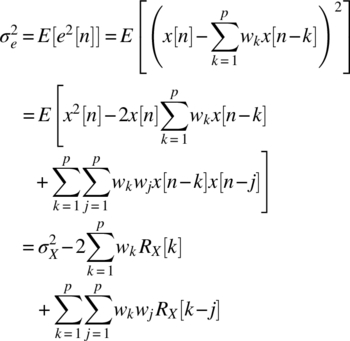
The power of nth sample x[n] (average input power to the prediction filter) is given by
where the mean value of x[n] is equal to zero. The autocorrelation of x[n] is defined by
The variance of the prediction error may be minimized (the so‐called minimum mean square error, mmse) by differentiating ![]() in (5.70) with respect to wk and equating to zero:
in (5.70) with respect to wk and equating to zero:

The above is the so‐called Wiener‐Hopf equation for linear prediction. The p unknown filter coefficients w1, w2,…, wp can easily be found from p equations in (5.73). For this purpose, we write the Wiener‐Hopf equation in matrix form as
where

Optimum weight vector which minimizes the mean‐square error is given by
To find the minimum prediction error, we insert (5.73) into (5.70) and get

5.4.2.1 Linear Adaptive Prediction
Linear prediction requires the knowledge of the statistics of signal samples in terms of the autocorrelation function R[k], k = 0, 1,… p, where p is the prediction order. The accurate determination of R[k], k = 0, 1, …, p requires the statistics of sufficiently large number of bits. This is often accomplished, in time varying channels, by using a training sequence at periodic time intervals; this brings an overhead and decreases the effective data rate. Hence, in time varying channels, the values of R[k], k = 0, 1,… p need to be updated at time intervals shorter than the channel coherence time, that is defined as the maximum time interval during which the channel gain does not change appreciably. It might therefore be attractive to use an adaptive prediction algorithm, where the tap weights wk, k = 1, 2,.. p are computed in a recursive manner, starting from some arbitrary initial values, without needing the statistics of R[k] but using only the instantaneously available data.
The adaptive prediction algorithm aims to minimize ![]() , which corresponds to the minimum point of the bowl‐shaped error surface that describes the dependence of
, which corresponds to the minimum point of the bowl‐shaped error surface that describes the dependence of ![]() on the tap weights. Successive (iterative) adjustments to the tap‐weights are made in the direction of the steepest descent of the error surface, that is, in the opposite direction of the gradient, where
on the tap weights. Successive (iterative) adjustments to the tap‐weights are made in the direction of the steepest descent of the error surface, that is, in the opposite direction of the gradient, where ![]() shows fastest decrease. The gradient of
shows fastest decrease. The gradient of ![]() in the directions of wk may be written as
in the directions of wk may be written as

By using ![]() , given by (5.70), one may express gk as follows:
, given by (5.70), one may express gk as follows:

In view of (5.73), the Wiener‐Hopf equation for linear prediction, (5.94) vanishes. However, the use of instantaneous values as estimates of the autocorrelation function facilitates the adaptive process:
where the prediction error at n‐th iteration is defined as

Here ![]() denotes the estimate of the j‐th tap weight at n‐th iteration. In view of the above, after sufficiently large number of iterations (5.95) and (5.96) are expected to be minimized. This implies that the tap weights are determined with sufficient accuracy so that the error signal vanishes.
denotes the estimate of the j‐th tap weight at n‐th iteration. In view of the above, after sufficiently large number of iterations (5.95) and (5.96) are expected to be minimized. This implies that the tap weights are determined with sufficient accuracy so that the error signal vanishes.
The kth tap weight at (n + 1)th iteration may be expressed in terms of its value at nth iteration wk[n], the step size μ and the prediction error as follows:

The iterative approach described above to determine the tap weights decreases the mean square prediction error in the direction of the steepest descent. The step‐size μ controls the speed of adaptation. Small μ implies slow convergence and poor tracking performance but more accuracy, while large μ implies rapid convergence but large variations around the optimum values of the tap weights, hence larger prediction error. The iteration stops either after a certain number of iterations or when the change in a tap weight between nth and (n + 1)th iteration becomes smaller than a predetermined value. Then, the variance of the prediction error remains in the near vicinity of its minimum value. The speed of convergence is required to be faster than the time rate of change of the channel gain so that the predictor can follow the random time variations in the channel. Depending on the channel coherence time, this may require fast DSP chips and algorithms. Periodic updates of the tap weights enable an adaptive predictor to correctly predict the desired signal sample with a reasonable number of iterations.
The block diagram of a linear adaptive predictor using least‐mean‐square (LMS) algorithm is shown in Figure 5.40. The input sample is predicted by a predictor using p previous samples of the same signal. The error signal, determined by difference between the current signal sample and its prediction, is then multiplied with x[n‐k] to determine the next iteration of the k‐th tap weight. Repeating this for all taps in all iterations minimizes the error signal in the mean square sense and predicts the current signal sample to be used for differential encoding in Figure 5.37.

Figure 5.40 Block Diagram of a Linear Adaptive Prediction Process.
5.4.3 Differential PCM (DPCM)
DPCM consists of transmitting the prediction error, difference between the actual signal sample and its prediction, as given by (5.69), after quantization (see Figure 5.41). The variance of the error signal is known to be smaller than the variance of the input sample itself (see Figure 5.38 and Example 5.12). Consequently, lower number of quantization levels L, hence fewer bits per sample, may be used to transmit the same signal. Therefore, DPCM allows lower transmission rates and bandwidths.[6]
Figure 5.41 shows the block diagram of a DPCM transceiver. At the transmitter, the signal at the quantizer input is the prediction error, ![]() , that is, the difference between the input sample x[n] and its prediction
, that is, the difference between the input sample x[n] and its prediction ![]() provided by the prediction filter. The prediction error, which is quantized and encoded before transmission, may be reduced by using a predictor with higher prediction order. If prediction is sufficiently good, the variance
provided by the prediction filter. The prediction error, which is quantized and encoded before transmission, may be reduced by using a predictor with higher prediction order. If prediction is sufficiently good, the variance ![]() of e[n] will be less than the variance
of e[n] will be less than the variance ![]() of x[n], which is simply the input signal power. Note that the simplest prediction filter is a single delay element (a single‐tap filter, p = 1), predicting the present sample as the previous one.
of x[n], which is simply the input signal power. Note that the simplest prediction filter is a single delay element (a single‐tap filter, p = 1), predicting the present sample as the previous one.

Figure 5.41 Block Diagrams of DPCM Transmitter and Receiver.
The quantizer output may be written as the sum of the error signal e[n] and the quantization error q[n]:
The quantization error q[n] will be decreased as the number of quantization levels, L, increases. Multilevel quantization of the error signal provides better information for message reconstruction at the receiver. However, with increasing L, the number of bits per sample, ![]() , and the required transmission rate,
, and the required transmission rate, ![]() , will increase. Note that the predictor provides a prediction
, will increase. Note that the predictor provides a prediction ![]() for the n‐th signal sample x[n] by using xq[n], the quantized version of the nth signal sample, and the quantized error signal:
for the n‐th signal sample x[n] by using xq[n], the quantized version of the nth signal sample, and the quantized error signal:

It is evident from (5.99) that xq[n] differs from x[n] only by the irrecoverable quantization error q[n] of the error signal. At the receiver, the decoded quantized error signal is added to the prediction filter output to regenerate the quantized signal sample. The same prediction filter as in the transmitter is used to predict a signal sample from its past values. In the absence of the channel noise, the signal at receiver output xq [n] differs from the signal sample x[n] only by the quantization error.
A quantizer can be designed to produce a quantization error with variance, ![]() , that is smaller than in the standard PCM by choosing a suitable value for the number of quantization levels L. Output SNR of DPCM may be expressed in terms of the variance of the prediction error as
, that is smaller than in the standard PCM by choosing a suitable value for the number of quantization levels L. Output SNR of DPCM may be expressed in terms of the variance of the prediction error as

where ![]() denotes the variance of the input sample x[n],
denotes the variance of the input sample x[n], ![]() is the variance of the quantization error q[n] and
is the variance of the quantization error q[n] and ![]() the variance of the prediction error. According to (5.19), the signal‐to‐quantization noise ratio is given by
the variance of the prediction error. According to (5.19), the signal‐to‐quantization noise ratio is given by ![]() . The processing gain Gp due to differential quantization
. The processing gain Gp due to differential quantization

provides an SNR advantage to DPCM over standard PCM in the order of 5–10 dB for voice signals. [6]
The error ![]() is proportional to the derivative of the input signal. Since
is proportional to the derivative of the input signal. Since ![]() changes as much as ± (L‐1)Δ from sample to sample (see Table 5.6), the maximum rate of increase of the error signal
changes as much as ± (L‐1)Δ from sample to sample (see Table 5.6), the maximum rate of increase of the error signal ![]() should be at least as fast as the input sequence of samples {x[n]} in a region of maximum slope. Hence, the DPCM signal should satisfy the following slope tracking condition:
should be at least as fast as the input sequence of samples {x[n]} in a region of maximum slope. Hence, the DPCM signal should satisfy the following slope tracking condition:

where fs = 1/Ts is the sampling frequency and Δ is the step size. Otherwise, Δ may be too small for the error signal to follow a steep segment of the input signal x(t); then we suffer the so‐called slope overload distortion. On the other hand, when the step size Δ is too large relative to local slope of input signal x(t), granular noise causes oscillations around relatively flat segments of signal samples. Since small values of the step size causes slope overload distortion, while large values of it is the source of granular noise, one should seek for an optimum step size which provides a trade‐off between the slope overload distortion and the granular noise.
5.4.4 Delta Modulation
Delta modulation (DM) is basically a special case of DPCM with three fundamental differences. In the block diagram of DPCM shown in Figure 5.41:
- The message signal is oversampled (higher than Nyquist rate) to purposely increase the correlation between adjacent samples. The rationale behind oversampling is to ensure that adjacent samples do not differ from each other significantly.
- The predictor has a prediction order p = 1 (single‐tap) in DM but p ≥ 2 for DPCM (multi‐tap). Since we have
 at the output of the single‐tap predictor, the error signal defined by (5.69) may be rewritten as
The quantized sample xq[n] in DM differs from the original sample x[n] by the quantization error q[n] as defined by (5.99).
at the output of the single‐tap predictor, the error signal defined by (5.69) may be rewritten as
The quantized sample xq[n] in DM differs from the original sample x[n] by the quantization error q[n] as defined by (5.99). - The error signal e[n] in (5.103) is quantized with one‐bit; the quantization level is L = 2 for DM compared to multilevel (L > 2) quantization in DPCM. As also shown in Figure 5.42, depending on positive (representing bit 1) and negative signs (representing bit 0) of e[n], the quantized error signal assumes one of two levels, ±Δ:
(5.104)


Figure 5.42 Delta Modulation.
DM provides a staircase approximation to the oversampled version of the message signal and achieves digital transmission of analog signals using a much simpler hardware than PCM. Since each sample is quantized with one bit, transmission rate in DM is equal to the sampling rate fs = 1/Ts, which is chosen to be much higher than the Nyquist rate, fs = 2 W. Table 5.7 shows the process of DM of the following sample sequence: x[1] = 0.9, x[3] = 0.3, x[4] = 1.2, x[5] = −0.2, x[6] = −0.8.
Table 5.7 The Steps for Delta Modulating the Sample Sequence {x[1] = 0.9, x[3] = 0.3, x[4] = 1.2, x[5] = −0.2, x[6] = −0.8}.
| n | x[n] | eq[n] | |||
| 1 | 0.9 | 0 (ref.) | +0.9 | +1 | 1 |
| 2 | 0.3 | 1 | −0.7 | −1 | 0 |
| 3 | 1.2 | 0 | +1.2 | +1 | 1 |
| 4 | −0.2 | 1 | −1.2 | −1 | 0 |
| 5 | −0.8 | 0 | −0.8 | −1 | −1 |
In a DM receiver, the quantized error signal is added to the one‐tap predictor output successively so that the n‐th sample of the quantized signal is found as follows:

Thus, at the n‐th sampling instant, the accumulator increments the predictor output by ∆ in positive or negative direction depending on the sign of eq[n]. The staircase approximation xq(t) is reconstructed by passing the sequence of positive/negative pulses, produced at the decoder output, through an accumulator in a manner similar to that used at the transmitter. Note that (5.105) is the digital equivalent of integration, since it represents the accumulation of positive and negative increments of the step size ∆. Out‐of‐band quantization noise in xq(t) is rejected by passing it through a LPF, of a bandwidth equal to the message bandwidth.
5.4.4.1 Slope‐Overload Distortion
In view of (5.99) and (5.103), the error signal at the quantizer input may also be written as
Ignoring the quantization error q[n‐1], the error signal is proportional to the derivative of the input signal. Since the maximum rate of increase of the error signal is Δ/Ts and occurs with a sequence of Δ’s of the same polarity (see Figure 5.43), the sequence {xq[n]} can increase faster than the input sequence of samples {x[n]} in a region of maximum slope if


Figure 5.43 Slope Overload Distortion and Granular Noise in Delta Modulation.
Otherwise, the slope Δ/Ts of xq(t) cannot follow a steep segment of the input signal x(t); this leads to slope overload distortion as shown in Figure 5.43.
5.4.4.2 Granular Noise
If the signal does not change too rapidly from sample to sample, xq[n] remains within ±Δ of the input sample x[n]. If the step size Δ is chosen much larger than the local slope of input signal x(t), then staircase approximation xq(t) induces oscillations around relatively flat segments of x(t). Therefore, as in DPCM, an optimum step size is needed so as to compromise the slope overload distortion and the granular noise. The optimum value of the step size maximizes the output SNR of a delta modulator. On the other hand, choice of very small values of Ts (large sampling frequency, fs) for preventing slope overload distortion is undesirable since it increases the transmission rate. Therefore, one may change the step size adaptively depending on the local slope of the signal.
5.4.4.3 Adaptive Delta Modulation (ADM)
ADM comprises an additional hardware, compared to DM, designed to provide variable step size, thereby reducing slope overload effects without increasing the granular noise. Slope overload appears in eq[n] as a sequence of pulses having the same polarity, whereas granular noise occurs when the polarity tends to alternate when xq(t) tracks x(t).
As shown in Figure 5.44a, which shows the block diagram of an ADM, the step‐size controller adjusts the variable gain g(n), so that (5.105) is modified as
where the step size is adaptively determined as follows:


Figure 5.44 Adaptive Delta Modulation (ADM).
Here, K is a constant in the range 1 < K < 2. In view of (5.110) and (5.111), the effective step size increases in discrete steps by successive powers of K during slope overload conditions. Variable step size yields a wider dynamic range. The SNR of ADM is typically 8–14 dB better than ordinary DM and the transmission bandwidth for voice is typically 24–32 kHz [6]. A scheme known as continuously variable slope delta modulation (CVSD) provides a continuous range of step‐size adjustments instead of a set of discrete values as in (5.111). Consequently, CVSD has better performance than DM and ADM.
5.4.4.4 Delta‐Sigma Modulation (DΣM)
As can be observed from (5.106), the error signal at the quantizer input of a DM is proportional to the derivative of the message signal. This leads to accumulation of noise power in the demodulated signal due to the presence of accumulator (integrator) in the DM receiver (see Figure 5.41). This drawback can be overcome by integrating the message signal prior to DM at the transmitter as shown in Figure 5.45. By integration at the transmitter, the low‐frequency content of the input signal is pre‐emphasized and the correlation between adjacent samples of the DM input is increased. The overall system performance is thus improved by reducing the variance of the error signal at the quantizer input and, at the same time, the receiver design is simplified.

Figure 5.45 Two Equivalent Block Diagrams of the Transceiver of a Delta Sigma Modulation System.
The so‐called delta‐sigma modulation (DΣM) is a version of DM that incorporates integration at its input. Since integration at the transmitter input should be compensated for by differentiation at the receiver, this need is satisfied by simply removing the integrator in the conventional DM receiver. Thus, as shown in Figure 5.45, the receiver of a DΣM consists only of a LPF.
Simplicity of implementation of the DΣM transceiver is achieved at the expense of sampling rates far in excess of that needed for PCM, hence increased transmission bandwidth. Then, one may use, for example, a multi‐tap prediction filter as in DPCM in order to reduce the transmission bandwidth.
5.4.5 Audio Coding
A voice signal, bandlimited to 3.4 kHz, sampled at 8 ksamples/s and quantizated with 8‐bits, is transmitted at 64 kbps. This rate is unacceptably high for some applications that require much lower data rates.
The speech process starts with the generation of a tone in the vocal chords. The throat, mouth, tongue, lips, and nose, and so on, acting as filters, modulate the generated tone. The speech signal consists of active periods separated by unvoiced time intervals. Unvoiced speech is modelled by white noise. Voiced speech may be modelled by periodic sequence of impulses with period which is equal to the reciprocal of the pitch frequency. Figure 5.46 shows a model for the generation of speech signals.
N samples of a speech signal are predicted as

where wn denotes the input sequence (white noise or impulses), G is the amplifier gain, {ai} are the tap gains and p denotes the prediction order. The first part in (5.112) represents the output of a prediction filter with p taps as shown in Figure 5.37. However the term Gwn does not depend on the previous speech samples. Linear prediction is used to determine the tap gains {ai}, as outlined in Section 5.4.2. For the optimal choice of the predictor coefficients, the mean square value of the prediction error may be written as

Figure 5.46 Block Diagram of a Speech Synthesizer.
When the excitation coefficients are normalized to unity, then the gain G is given by [2]

Linear predictive coding (LPC) provides an alternative approach to digital transmission of analog voice signals compared to the classical approach, which is based on ADC of the analog voice signals. LPC is based on extracting the parameters of a voice signal, for every 10‐25 ms, and transmitting this information with a prespecified number of bits. A transversal filter and some auxiliary components are used to extract the required signal parameters, for example, volume and the duration of the tone, pitch frequency, and so on, and the tap weights of the transversal filter. [2][6] As shown in Figure 5.47, voice samples are analyzed to determine the parameters for the synthesizer. The error signal, defined as the difference between the input and synthesizer output, is encoded along with these parameters for transmission. These parameters and the quantized error signal are used by the receiver to regenerate the original speech signal.
A complete LPC codeword consists of typically 80 bits accounting for pitch frequency, amplifier gain, tap weights of the transversal filter, and so on. Updating the parameters every 10‐25 ms is equivalent to sampling at 40‐100 Hz. So, LPC requires very modest bit rates in the range of 3.2 kbps (80 bits/25 ms)‐8 kbps (80 bits/ 10 ms). [6] Therefore, LPC is very effective for digital voice transmission and is currently employed in many modern communication systems.

Figure 5.47 Block Diagram of a LPC Transceiver.
The GSM system uses regular pulse excited long‐term prediction (RPE‐LTP) coding, which is based on PLC. ADC of speech signals at 8 ksamples/s and 13 bits/sample leads to a bit rate 104 kbps at the RTP‐LTP encoder input. Based on the observation that the speech signals are approximately constant during 20 ms intervals, the filter parameters characterizing a speech signal are updated with 20 ms intervals. This corresponds to sampling speech signal at 1/20 ms = 50 samples/s; such low sampling rates provide a compromise between the speech quality and the bit rate. In the RPE‐LPT algorithm, features of each 20 ms speech block are extracted, and encoded into 260 bits with a net bit rate of 260 bits/20 ms = 13 kbits/s. Hence, a RTP‐LTP encoder reduces the input bit rate of 104 kbps to 13 kbps. Speech signals are then protected against channel errors with the addition of 196 redundancy bits, so that a total of 456 bits are transmitted during 20 ms interval with a channel rate of 456 bits/20 ms = 22.8 kbits/s. Note that this rate is approximately ~22% of 104 kbps obtained using ADC.
The adaptive multi‐rate (AMR) is a multi‐rate narrowband audio compression format optimized for speech coding. It is based on 160 bits for 20 ms frames, and narrowband (200–3400 Hz) signals are encoded at variable bit rates ranging from 4.75 to 12.2 kbit/s. AMR was adopted as the standard speech codec by 3GPP in October 1999 and is now widely used in GSM and UMTS. It adaptatively selects one of eight different bit rates (12.2, 10.2, 7.95, 7.40, 6.70, 5.90, 5.15 or 4.75 kbit/s) depending on the channel conditions. [7][8] Although AMR is basically a speech format and may not give ideal results for other audio signals, AMR codec is also used for storing short audio recordings in mobile telephone handsets. The AMR codec can also be used for applications like random access or synchronization with video.
5.4.6 Video Coding
Multimedia communications in many applications require transmission of audio, video and data signals at low data rates. We know from Example 5.5 that high data rates are needed to transmit digital video services unless video compression is used. As an integral part of video encoding, high compression ratios of video signals are strongly desired in various applications including TV broadcasting, videoconferencing, digital storage, internet streaming, and wireless communications.
Data compression drastically reduces the transmission rate and enables efficient storage and transmission of multimedia signals. Lossless data compression (data compaction) is reversible and operates as ZIP codes used to compress document files. The objective of lossless data compression is to map the original bit stream into a shorter stream, so that the original bit stream can be recovered exactly from the compressed stream. Lossy data compression is irreversible, and aims to compress the original data at the expense of some degradation.
Video compression is possible due to the fact that adjacent parts of a single video frame as well as successive frames are similar to each other. Therefore, transmitting the differences between scenes within the frame and between adjacent frames is much more economical than transmission of all the frames. The interframe redundancy can be significantly reduced to produce a more efficiently compressed video signal. This reduction is achieved through the use of prediction of each frame from its neighbors; the resulting prediction error (differential encoding) is transmitted for motion estimation and compensation. In brief, video compression algorithms exploit two types of redundancy in the signal: temporal (changes from one frame to the next) and spatial (changes in the pixels within one frame). Still image coding algorithms like Joint Photographic Experts Group (JPEG) only exploit the spatial redundancy.
Video compression techniques include
- Discrete cosine transform (DCT), which is a frequency transform technique similar to Fourier Transform, is used to reduce the spatial redundancy in video frames.
- Quantization is a technique for deliberately losing some information (lossy compression) from the pictures.
- Huffman coding, run length coding, and variable length coding are lossless compression techniques and use code tables based on the data statistics to encode more frequently encountered data with shorter codewords.
- Motion compensated predictive coding aims to exploit temporal redundancy. The differences (changes) between current and preceeding frames are calculated and encoded.
- Bi‐directional prediction where some images are predicted from the pictures immediately preceding and following the image.
The first three of the above compression techniques are also used by the JPEG standard, which was developed for compressing full‐color or greyscale images of natural, real‐world scenes by exploiting known limitations of the human visual system. Low resolution pictures such as computer generated images can be transmitted or stored at data rates up to 1.5 Mbps.
Motion Photographic Experts Group (MPEG‐1) standard was initially designed to primarily compress video‐CD (non‐interlaced video) images of size 352 × 288 at 25 frames/s at a transmission rate of 1.5 Mbps. In contrast with JPEG, MPEG‐1 exploits the interframe (temporal) redundancy and provides motion‐compensated compression. [9]
MPEG‐2 standard, published in 1995, was designed for coding standard‐definition (SD) 4:2:0 video at bit rates 3‐6 Mbit/s, with a drastic reduction from ~144 Mbps. MPEG‐2, used for digital TV broadcast and DVD, has many features in common with MPEG‐1 and achieve compressing ratios up to 50:1.
MPEG‐3, launched mainly for the HDTV applications, refers to a group of audio and video coding standards designed to handle HDTV signals at 1080p (p stands for progressive scanning) in the range of 20 to 40 Mbps. However, as MPEG‐2 was observed to have the ability to accommodate HDTV services as well, HDTV was included in 1992 as a separate profile in the MPEG‐2 standard.
MPEG‐4, though initially introduced in 1998 for low bit‐rate video communications, is efficient across a variety of bit‐rates ranging from a few kbps to tens of Mbps. MPEG‐4 provides improved coding efficiency over MPEG‐2, ability to encode multimedia data (video, audio, speech), and robustness against errors. For MPEG‐4, bit rates as low as 2 Mbp/s is considered to provide a good compromise between picture quality and transmission bandwidth efficiency. MPEG‐4 addresses speech and video synthesis, fractal geometry, computer visualisation, and an artificial intelligence approach for reconstructing images.
ITU‐T H.264/MPEG‐4 Advanced video coding (AVC) standard, which is published in 2003, allows broadcasting over cable, satellite, cable modem, terrestrial, and so on. Using H.264/AVC, it is possible to transmit video signals at about 1 Mbps with PAL quality, which enables streaming over xDSL connections. H.264 standard contains a set of video coding tools but not all of them are needed for every application. A H.264 decoder may choose to implement any number of them depending on the needs of the application. The adoption of H.264 standard led to doubling the number of TV programmes per satellite in comparison to the use of H.262 (MPEG‐2). H.262 also allows
- Interactive or serial storage multimedia on DVD, optical and magnetic devices,
- Videoconferencing and videophone,
- Video‐on‐demand and multimedia streaming services,
- Multimedia messaging services, and
- Multimedia services over packet services, such as multimedia mailing.
High efficiency video coding (HEVC) standard was published in 2013. It aims to achieve a factor of two improvement in compression efficiency compared to the H.264/AVC standard. HEVC is a strong candidate for new generation digital TV services using 1080p.
Figure 5.48 shows the milestones in the evolution of the bit rate required for the transmission of HD(1080p) TV signals. One may easily observe drastic decrease of the required bit rates in this rapidly evolving area.
Figure 5.48 Evolution of Video Coding Standards with Time for HD (1080p) TV. [9]
References
- [1] S. Haykin, Communication Systems (3rd ed.), J. Wiley: New York, 1978.
- [2] J. G. Proakis and M. Salahi, Communication Systems Engineering (2nd ed.), Prentice Hall: New Jersey, 2002.
- [3] N. Judell, and L. Scharf, A simple derivation of Lloyd’s classical result for the optimum scalar quantizer, IEEE Trans. Information Theory, vol. 32, no. 2, pp. 326–328, 1986.
- [4] N. S. Jayant, and P. Noll, Digital Coding of Waveforms, Principles and Applications to Speech and Video. Prentice Hall, New Jersey, 1984, pp. 115–251.
- [5] Z. Peric, and J. Nikolic, An effective method for initialization of Lloyd‐Max’s algorithm of optimal scalar quantization for Laplace source, Informatica, vol. 18, no. 2, pp. 279–288, 2007.
- [6] A. B. Carlson, P. B. Crilly, and J. C. Rutledge, Communication Systems (4th ed.), McGraw Hill, Boston, 2002.
- [7] 3GPP TS 26.071 Mandatory speech CODEC speech processing functions; AMR speech Codec; General description.
- [8] 3GPP TS 26.090 Mandatory Speech Codec speech processing functions; Adaptive Multi‐Rate (AMR) speech codec; Transcoding functions.
- [9] K. McCann, Future Codes, Progress Towards High Efficiency Video Coding, DVB Scene 39 March 2012, p. 5, https://www.dvb.org/
Problems
- 1. The zero‐order hold circuit, shown in Figure 5.8, is not only used for flat‐top sampling in ADCs but also in DACs to reconstruct signal x(t) from its samples with a sampling interval of Ts.
- Find the impulse response h(t) of this circuit.
- Find the transfer function H(f).
- Show that when a sampled signal
 is applied at the input of this circuit, the output is a staircase approximation of x(t).
- 2. A band‐limited signal having bandwidth W can be reconstructed by its samples as described by (5.6). Using the samples g − 1 = −1, g0 = 2, g1 = 1 and gn = 0 for n ≠ −1, 0, 1, plot the received signal as a function of time.
- 3. The information in an analog voltage waveform, bandlimited to 3.4 kHz, is to be transmitted using 16‐PCM. The quantization error is specified not to exceed 0.1 % of the peak‐to‐peak analog signal.
- Determine the minimum number of bits per sample that meets the distortion requirements.
- Determine the signal to quantization noise ratio for PAPR = 6 dB.
- Determine the minimum required sampling rate, and the resulting bit rate.
- Determine the symbol rate for binary PCM.
- What is the transmission rate if 16‐ary PAM transmission is used instead of the binary PCM?
- 4. The quantization error in a PCM system is required not to exceed 1% of the peak‐to‐peak analog signal voltage.
- Determine the bandwidth efficiency (bits/s/Hz) of a speech signal bandlimited to 3.4 kHz and sampled at the Nyquist rate.
- Repeat (a) for an (high fidelity) audio signal bandlimited to 20 kHz.
- 5. A compact disc (CD) recording system samples each of two stereo signals with a 16‐bit ADC at 44.1 kilosamples/s.
- Determine the average output signal‐to‐quantization noise ratio for PAPR = 1.
- If the recorded music is designed to have a PAPR = 20, determine the average output signal‐to‐quantization noise ratio.
- The bit stream at the ADC output is augmented by error‐correcting bits, bits for clock extraction and display and control. These additional bits represent 100% overhead, the bit rate at ADC output is doubled. Determine the output bit rate of this CD recorder system.
- If the CD can record 75 minutes of music, determine the number of bits recorded on a CD.
- Consider a book of 1500 pages, 100 lines/page, 15 words/line, 6 letters/word, and 6 bits/letter. Determine the number of bits required to store the book and estimate the number of comparable books that can be stored on a CD.
- 6. A music signal has a bandwidth of 20 kHz and a PAPR of 20 dB. Calculate the bit rate required to transmit this as a linearly quantised PCM signal with a SNRQ = 50 dB. Assuming that the minimum ISI‐free PCM bandwidth is given ½ of the transmission rate, determine the minimum required transmission bandwidth.
- 7. An overall SNR of 53 dB is required for the reconstructed analog signal to achieve a bit error rate of 10−6 in a uniformly quantized PCM system. The analog signal is modeled by a stationary random process whose average power is 16 W.
- Determine the corresponding signal‐to‐quantization noise ratio, SNRQ, and the number of quantization levels?
- Assuming that the signal is quantized to satisfy the condition of part (a) and assuming the approximate bandwidth of the signal is W = 4 kHz, determine the bit rate of a binary PCM signal based on this quantization scheme?
- 8. A signal varying between ±4V is sampled 10 ksamples/s and is uniformly quantized using 8 bits.
- Determine the maximum quantization error.
- Determine the average quantization noise power.
- Determine the number of bits/sample needed to reduce the maximum quantization error to 10 mV.
- Discuss the costs associated with the quantization error reduction achieved in part (c).
- 9. Consider that an analog signal is sampled at 8 ksamples/s, quantized with 3 bits/sample, and Gray encoded as shown below.

- Determine the sampling interval and calibrate the x‐axis in the figure above.
- Determine the data sequence if uniform quantization is used.
- Determine the data sequence if μ‐law companding is used with μ = 50. Estimate the original values of the samples by inspecting the waveform.
- Compared with uniform quantization, what are the advantages and disadvantages of nonuniform quantization?
- 10. Consider that an audio signal bandlimited to 4 kHz is sampled at 8 k samples/s. Assuming that the ratio of peak signal power to average quantization noise power at the output does not exceed 40 dB:
- Determine the minimum number of bits/sample needed for uniform quantization.
- Determine the bit rate.
- Determine the null‐to‐null bandwidth of this PCM signal using polar NRZ line code.
- 11. The signal x(t) = 8 cos(20πt) is sampled at a rate 50 samples/s, uniformly quantized and encoded with 4 bits.
- Determine the values of the 16 representation levels and establish the correspondence between representation levels and Gray‐encoded 4‐bit symbols.
- Insert the uniformly quantized values and the corresponding 4‐bit symbols in the table below for the non‐companded signal.
Sample Number x[n] Xq[n] 4‐bit symbol 0 1 2 3 4 5 - Determine the normalized RMS quantization error averaged over one cycle, by using the following formula, where N is the number of samples in one cycle of the signal.

- Now consider that a compander described by
 is used for non‐uniformly quantizing the signal x(t). Determine the non‐uniformly quantized values and insert them and the corresponding 4‐bit symbols into the table below.
Sample Number x[n] y[n] yq[n] 4‐bit symbol 0 1 2 3 4 5 - Determine the normalized RMS quantization error averaged over one cycle for the companded signal.
- Compare the results obtained in (c) and (e).
- Show that, without quantization, we get the original signal if we use an expander, as described by
 where y[n] denotes the input to the expander.
- 12. A random variable X with pdf
 is quantized using a 3‐level quantizer with output y specified as
where 0 ≤ Δ ≤ a.
is quantized using a 3‐level quantizer with output y specified as
where 0 ≤ Δ ≤ a.
- Derive an expression for the resulting mean–squared error (MSE)
 in terms of a and b.
 - Determine the optimal values of a and Δ that minimize the MSE and the minimum value of
 .
. - Determine the average signal power to quantization noise power ratio.
- Derive an expression for the resulting mean–squared error (MSE)
- 13. Repeat Problem 5.12 for a 4‐level quantizer with output y specified as
where 0 < a < Δ < b.

- Derive an expression for the resulting mean–squared error (MSE)
 in terms of a, b and Δ.
 - Find the optimal values of a, b and c such that MSE is minimized. Determine the minimum value of
 .
. - Determine the average signal power to quantization noise power ratio. Compare your results with those of Example 5.8.
- Derive an expression for the resulting mean–squared error (MSE)
- 14. A scanner is used to scan images of A4 page (size 210 mm 297 mm) into a data file using 8 bits/pixel (pixel denotes picture element). It takes 100 ms to transmit the data file created by scanning at a transmission rate of 1 Mbps. Determine the resolution of the scanner, that is, number of pixels used per cm2?
- 15. Consider a uniform quantizer as shown in Figure 5.12. Assume that a Gaussian‐distributed random variable with zero mean and unit variance is applied to this quantizer input.
- Find the probability density function of the discrete random variable at the quantizer output.
- Determine the quantization noise power and the signal‐to‐quantization noise power ratio, and compare your results with that obtained for uniform and Laplace distributions (see Example 5.7).
- 16. A PCM system uses Nyquist sampling, uniform quantization and 8‐bit encoding. The bit rate of the system is equal to 20 Mbps.
- What is the maximum message bandwidth for which the system operates satisfactorily when the message signal is sampled at the Nyquist rate?
- Determine the output signal‐to‐quantizing noise ratio for an input sinusoidal modulating wave.
- 17. A 8‐bit ADC with uniform quantizer is designed to operate over ±4 V.
- Determine the step size.
- Determine the signal‐to‐quantization noise ratio for a uniformly distributed random signal.
- Determine the signal‐to‐quantization noise ratio for a Gaussian signal with variance σ2, where the signal voltage is limited to ±4σ.
- Determine the probability of signal saturation in part (c).
- 18. The dynamic range of a signal x(t), whose amplitude is limited by ±xmax, is defined as
This definition is meaningful since minimum signal power level may approach zero, but the noise is always present. In PCM, the average noise power level is determined by the quantization noise power since it dominates the Gaussian noise. Determine the number of bits required for an ADC to encode music with a dynamic range higher than 120 dB.

- 19. A message signal with ±1V peak voltage is transmitted using binary PCM with uniform quantization. The average message power equals 20 mW over a 1 Ohm resistance. If the signal‐to‐quantization‐noise ratio (SNRQ) is required to be at least 46 dB:
- Determine the minimum number of bits per sample and the corresponding number of quantization levels.
- Determine the SNRQ actually obtained with this quantizer.
- If the bit error probability of the channel is 10−6, then calculate the SNR in dB at the decoder output.
- 20. A TV signal, m(t), bandlimited to 4.5 MHz is to be transmitted by binary PCM. The receiver output signal‐to‐quantization‐noise ratio is required to be at least 55 dB.
- If all brightness levels are assumed to be equally likely, that is, amplitude of m(t) is uniformly distributed in the range (−mmax, mmax), determine the minimum required number of quantization levels L, and the corresponding bit rate.
- For this value of L, determine the signal‐to‐quantization noise power ratio SNRQ.
- If the output SNRQ is required to be increased by 6 dB, what is the new value of L and the corresponding transmission bandwidth?
- Repeat b) and c) for 8‐level PCM
- 21. Oversampling implies sampling rates higher than the Nyquist rate, fN = 2W of a signal bandlimited to W. Oversampling ratio (OSR) is defined as the real sampling rate to the Nyquist rate:
 . Oversampled signal evidently occupies a bandwidth larger than W.
- Write down the PSD of a quantization noise, bearing in mind that the PSD means the mean power per unit bandwidth.
- Write down the total amount of quantization noise power in the signal bandwidth W in terms of the OSR.
- If Nyquist‐sampled and oversampled signals have the same signal‐to‐quantization‐noise power ratios, determine the increase in the resolution of an R‐bit convertor due to oversampling. Calculate this increase for OSR = 1.2.
- 22. Consider a bandpass signal which has a spectrum as shown below with a bandwidth B = fU‐fL Hz, where fU and fL denote upper and lower frequencies, respectively. According to the bandpass sampling theorem, a bandpass signal can be recovered from its samples by bandpass filtering if the sampling frequency is selected as fs = 2fu/K where K is the largest integer not exceeding fu/B. All higher sampling rates are not necessarily usable unless they exceed 2fu.
Assuming B = 10 KHz and fu = 25 kHz:
- Plot the spectrum of the sampled signal for the sampling frequencies 25 kHz, 40 kHz, and 50 kHz,
- Verify the bandpass sampling theorem by observing whether and how the sampled signal can be recovered for these three sampling frequencies,
- Compare your results with those of Example 5.4, where a bandpass signal is down‐converted to baseband before baseband sampling.

- 23. Derive the autocorrelation function and the PSD of NRZ bipolar codes in Table 5.4.
- 24. Determine and plot the power spectrum of a sequence
of independent and equiprobable message bits bk = ±1.

- Obtain the PSD using the following definition of the Manchester line code
where T denotes the bit duration and


- Derive the autocorrelation function given in Table 5.4 and then obtain the PSD.
- Obtain the PSD using the following definition of the Manchester line code
- 25. Draw the pulse stream for the bit stream {11000101} line codes for unipolar NRZ, bipolar NRZ, and Manchester code.
- 26. Consider that a line code given by
is used to transmit a bit sequence {bk} as follows:
 where
where
 have equal probabilities of transmission and T denotes the bit duration. Determine the power spectral density (PSD) of s(t) by clearly showing all the necessary steps.
 - 27. Consider the unipolar RZ and bipolar RZ binary signaling with bit duration T, as shown below for the binary data stream 110101. Determine the power spectral density (PSD) of these line codes by clearly showing all the necessary steps.

- 28. Several audio channels with W = 20 kHz are to be transmitted via binary PCM with R = 12 bits/sample.
- Determine how many of the PCM signals can be accommodated by the first level of the E1 multiplexing hierarchy.
- Calculate the corresponding bandwidth efficiency, which is defined as the ratio of transmission bandwidth of the PCM signal to that for the analog transmission (frequency division multiplexing) with single‐sideband (SSB). Assume that the minimum ISI‐free PCM bandwidth is given ½ of the transmission rate.
- 29. A TDM carrier supports a frame structure which consists of 30 voice channels, bandlimited to 4 kHz, sampled at Nyquist rate and encoded with 6‐bits/samples. Assuming that the frame uses 1 synchronization bit per channel and 1 synchronization bit per frame, determine the required data and frame rates.
- 30. Ten message signals, each having 2 kHz bandwidth, are time‐division multiplexed using uniformly quantized binary PCM. The sampling rate is 20 % higher than the Nyquist rate. The quantization error cannot be exceed 1% of the peak amplitude.
- Determine the number of quantization levels and the number of bits per sample.
- Determine the sampling rate.
- Determine the overall bit rate for the multiplexed signals.
- 31. Consider a TDM system with four signals, one of them bandlimited to 4 kHz and the remaining three signals are bandlimited to 2 kHz.
- Draw the block diagram of a time‐division multiplexer for multiplexing these signals, each sampled at their Nyquist rate.
- If the output of the multiplexer switch is quantized with 1024 levels and the result is binary‐coded, determine the output rate.
- 32. A TDMA system multiplexes 100 user signals each at 10 Mbps at the multiplexer input. Each user packer consists of 100 bits. A guard time of 1 bit duration is inserted between slots and a preamble of 250 bits used for address information, equalization, and so on.
- Determine the frame duration
- Determine the throughput efficiency of this multiplexer
- Determine the effective data rate at the TDM output.
- 33. Consider the first level E1 multiplexing hierarchy, where 30 voice signals each bandlimited to 4 kHz are sampled at Nyquist rate and encoded by 8 bits/sample. The multiplexed signals are transmitted at a rate of 2.048 Mbps.
- Determine the bit duration of the multiplexed signal and that of one of the 30 signals before multiplexing.
- If the bit amplitudes are ±1 Volt before multiplexing, determine the bit amplitude of multiplexed signal if the bit energy remains the same before and after multiplexing. Determine the corresponding increase in the transmit power of the multiplexed signal in dB.
- Determine the increase in the bandwidth of the multiplexed signal compared to that of a signal before multiplexing. Determine the percentage contribution of overheads to the bandwidth of the multiplexed signals.
- If the Eb/N0 of the multiplexed signal is chosen so as to achieve a bit error probability of 10−6, determine the average number of bit errors that may be observed in 10 seconds?
- 34. In an adaptive PCM system for speech coding, the input speech signal is sampled 160 times per 20 ms, and each sample is represented by 8 bits. The quantizer step size is recomputed every 10 ms, and it is encoded for transmission using 5 bits. In addition, 1 byte is added at the beginning of each packet (containing 160 voice samples) as header.
- Draw the packet structure showing the packet duration and the lengths in bits of the packet constituents.
- Compute the effective transmission bit rate of such a speech coder assuming that information and overhead bits are transmitted in 20 ms duration in real‐time applications.
- Determine the percentage increase in transmission rate due to overhead bits.
- 35. Show that
 and verify the bit error probability expression in (5.51).
 - 36. Consider a uniformly quantised signal with 8 bits over a noisy channel. What probability of bit error can be tolerated if the reconstructed signal is to have an SNR of 50 dB?
- 37. A stationary random process has an autocorrelation function given by
 where A is limited to ±4.
- When a μ‐law compander is used, show that the output signal‐to‐quantization noise ratio becomes
where R denotes the number of bits per sample and P denotes the average power of the message signal, whose amplitude is limited to ±A.

- Assuming A = 4, how many quantization levels are required to guarantee a signal to quantization noise power ratio of at least 50 dB?
- Assuming a companded PCM system with R = 8 bit and μ = 255, calculate the SNRQ in dB for very large and very small signal amplitudes and compare with the corresponding uniformly quantized PCM system.
- Repeat (c) for R = 8 bit and μ = 50.
- When a μ‐law compander is used, show that the output signal‐to‐quantization noise ratio becomes
- 38. The ramp signal x(t) = kt is applied to a delta modulator that operates with a sampling period T and step size Δ.
- How should T and Δ be chosen so that slope‐overload distortion does not occur.
- Sketch the DM modulator output for the following three values of step size: Δ = 0.75 kT,
- Δ = kT, and Δ = 1.25 kT.
- Discuss the implications of choosing larger/smaller values of T and Δ as long as the ratio Δ/T remains constant.
- 39. The signal waveform shown below is to be transmitted using DM at 10 kbps using a slope of ±5 volts/sec.

- Determine the value of Δ.
- Determine the DM bit stream.
- Draw the waveform that will appear at the output of the DM decoder prior to low‐pass filtering.
- 40. Consider a delta‐modulation system with a first‐order predictor, defined as
 where x[n] denotes the n‐th sample of a stationary signal of zero mean and the tap gain w1 is a constant. Assume that the energy of an antipodal signal is described by
  .
.
- Determine the optimal value of w1 which minimizes the prediction error in the mmse sense
 and find its minimum value.
 - Find the optimal prediction gain which is defined as the ratio of the average signal power to the minimum variance of the prediction error.
- If the variance of the prediction error is to be less than or equal to σ2, determine the condition that the channel tap must satisfy.
- Determine the optimal value of w1 which minimizes the prediction error in the mmse sense
- 41. Solve the three‐tap equalization problem in Example 5.13 using MSE approach, where the three tap coefficients are required to minimize the mean square value of the error (MSE) between the kth equalizer output sample yk and the kth data symbol, ak, that is,
 . Determine the tap coefficients and the minimum MSE for h0 = 1 and h1 = 0.3, and σ2 = 0.01. Compare your results with those found in Example 5.13.
 - 42. Consider a linear predictor with single tap.
- For optimal single‐tap prediction, determine the tap weight if the signal‐to‐prediction noise power ratio is 28 dB.
- If the signal‐to‐quantization noise ratio should be larger than 46 dB and peak‐to‐average power ratio is 10 dB, determine the required number of bits per sample.
- 43. Assuming that a voice signal can be approximated by a sinusoid of frequency f = 800 Hz, determine the sampling frequency required by DM for 256 quantization levels to meet the slope overload condition. Compare the sampling frequency you found with that required for PCM. Can DM provide an alternative to PCM?
- 44. Determine the tap gains, the minimum error variance, and the processing gain in dB for DPCM with a single‐tap and two‐tap prediction filter when the input signal is characterized by the autocorrelation R(0) = 1, R(1) = 0.9 and R(2) = 0.6.