
We can work with a lot of languages and tools in knitr, including but not limited to R, although knitr is an R package and has to be run within the R environment in the first place. Currently knitr supports Python, Ruby, Haskell, awk/gawk, sed, shell scripts, Perl, SAS, TikZ, Graphviz, and C++, etc. We have to install the corresponding software package in advance to use an engine.
Like chunk hooks, all language engines are essentially R functions in knitr. These functions pass the code chunk to external programs, run the code there, get the results back, and write to the output. In most cases, the code is passed to external programs via the system() function. For example, we can pass code to bash via the -c option.

For those who are not familiar with bash scripts, the code ls ~ | grep ˆD means to list files under the home directory (~) and pass the filenames to grep through the pipe ( | ) to match those starting with the letter D; ls and grep are standard Linux commands.
The chunk option engine can be used to specify the language engine for a chunk, e.g., the chunk below uses engine = ’bash’:

Then the code in the chunk will be treated as a bash script instead of an R script. The output rendering is similar to R output: the source code is passed to the source hook (i.e., knit_hooks$get(’source’)), and the output is passed to the output hook (knit_hooks$get(’output’)). The built-in output hooks are fairly general in terms of document formats; we do not need to think about whether the output is to be ![]() or HTML or Markdown; everything will be automatically and properly marked up according to the output document format.
or HTML or Markdown; everything will be automatically and properly marked up according to the output document format.
All language engines are stored in the object knit_engines, which has the $get() and $set() methods like knit_hooks (chunk hooks) and opts_chunk (chunk options); e.g., we can get the Python engine by knit_engines$get(’python’), or override the built-in Python engine by knit_engines$set(python = function(options) {…}).
An engine has one argument: options, which is a list of current chunk options. Among all options there is one special option named code, which is the code (as a character string) of the current chunk and plays the central role in the language engine.
To continue the bash example, we can define a preliminary engine like this:

What this engine does is to concatenate the command bash -c with the source code, execute the whole command via system(), and return both the source code and output as one character string separated by line breaks. The returned character string will be written into the output document.
The real bash engine is more complicated than this: it has to take care of some chunk options such as echo, results, include, cache, and so on. For example, when echo = FALSE, the source code should be hidden, and when cache = TRUE, the code chunk should be cached. In all, the behavior of these language engines is very similar to the R engine, although the support is not as comprehensive as R.
Note in particular the cache of language engines other than R: in most cases, only the side effects such as printing are cached, due to the fact that it is difficult for R to know which objects are created in a code chunk if the code is not written in R. In other words, objects are lost when we exit from a chunk (unless they are exported to files). Normally we will not be able to reuse an object created from previous chunks. The reason that we can use R objects across different chunks is that all R chunks are evaluated in the same R session, but other languages are evaluated in separate sessions per chunk basis.
For language engines, there are two common chunk options:
engine.path specifies the full path to the engine program as a character string; this may be useful to Windows users when the program to be called is not in the environmental variable PATH (i.e., the program cannot be run without full path in the command line), or to Linux users when there are multiple versions of one program installed and we do not want to use the default version; in both cases, we can set the chunk option engine.path = ’full/path/to/program’, e.g., engine.path = ’/usr/bin/ruby1.9.1’ (if there are multiple versions of Ruby) or engine.path = ’C:/Program Files/SASHome/x86/9.3/sas.exe’(to specify the full path of SAS);
engine.opts additional options to be passed to an engine; its value depends on the specific engine; for most engines, it contains additional command line arguments, e.g., for engine = ’ruby’, we can set engine.opts = ’-v’ for Ruby to print its version number, then turn on the verbose mode.
Most languages and tools are supported through the system() interface, as mentioned in the last section. There are a few exceptions, however, such as C++ and TikZ.
C++ is supported in knitr through the Rcpp package (Eddelbuettel et al., 2015). When we set engine = ’Rcpp’, the function sourceCpp() in Rcpp is used to compile C++ code chunks, which in fact calls R CMD SHLIB internally to build a shared library and load it into R for future use.
Below is an example for the Fibonacci series in C++ with Rcpp:

After it is compiled, we can call the function fibCpp() in R directly because we have marked it with the Rcpp::export attribute.

Below is the version implemented in pure R:

Unsurprisingly, the R version is much slower, although the numeric results are the same:

Finally, we can pass additional arguments to sourceCpp() via the chunk option engine.opts. For example, we can specify engine.opts = list(showOutput = TRUE) to show the output of R CMD SHLIB(note showOutput is an argument of sourceCpp()).
There are two simple language engines c and fortran for the C language and Fortran, respectively. These engines are nothing but wrappers for the command R CMD SHLIB and the R function dyn.load(). What they do is to write the code chunk to a temporary file, run R CMD SHLIB to compile it, and use dyn.load() to load the compiled library (a .dll or .so file). To use these engines, you have to make sure you have the C/Fortran compilers in your system, such as GCC.

Below are two examples demonstrating the usage of these two engines. First, we set the chunk option engine = ’c’ for this example:

After compiling the above code chunk, we can call the C function my_square() via the .C() interface:

![]()
Next, we show a Fortran example by setting the chunk option engine = ’fortran’ for the chunk below:
And we can call the Fortran sub-routine via the .Fortran() interface:

C++, C, and Fortran belong to compiled languages, and there are other languages that are interpreted languages. For these languages, we can execute the code without compiling it. Examples include awk and shell scripts. There are also some languages that belong to both categories, such as Python. Table 11.1 lists some interpreted languages supported by knitr via the system() interface.
For example, a Perl chunk is executed with perl -e code where code is the character string of the code chunk. For awk and sed, the argument after the program is treated as the source code, so they do not need an argument name for the code, e.g., awk ’END{print NR;}’ README counts the number of lines in the file README. For SAS, the code chunk is written into a file tempfile.sas, and executed as sas -SYSIN tempfile.sas. There are three shell variants: sh, bash, and zsh.
TABLE 11.1: Interpreted languages supported by knitr: the language name, engine name, and the command line argument to execute code.
Language |
Engine |
Code argument |
Python |
python |
-c |
Ruby |
ruby |
-e |
(g)awk |
(g)awk |
|
sed |
sed |
|
shell |
sh/bash/zsh |
-c |
Perl |
perl |
-e |
Haskell |
haskell |
-e |
CoffeeScript |
coffee |
-e |
Groovy |
groovy |
-e |
Node.js |
node |
-e |
Scala |
scala |
-e |
SAS |
sas |
-SYSIN |
As we mentioned before, the engine name itself may not be the executable, so we may need to specify the path to the real path of the program. For Haskell, haskell is not the program to run Haskell, whereas ghc is, so we need to specify both engine = ’haskell’ and engine.path = ’ghc’.
We give a few examples of the above languages. Here is a Python chunk (chunk option engine = ’python’):

Here is a Ruby chunk:

Below is an awk script to count the number of non-empty lines in the NEWS.Rd file of the knitr package: in awk, NF denotes the number of fields on a line; when it is not 0, the variable i increases by 1, and that is why the script counts the non-empty lines in the file. Note that we used engine.opts = shQuote(system.file(’NEWS.Rd’, package = ’knitr’)) for this chunk; i.e., we get the path to the NEWS.Rd file from R, quote it by shQuote(), and pass it to awk as the second argument (remember the first argument is the code chunk), which means the file to be read into awk.

Finally we have a Perl code chunk:

We can use the rstan package (Guo et al., 2014) to compile models of Stan, a relatively new programming language featuring Bayesian statistical inference. There is a language engine called stan in knitr that allows us to write Stan models in code chunks. We can certainly compile a Stan model in a normal R code chunk without using a special language engine, by saving the model as a file, or writing the model as a long character string in R code. Both ways have their disadvantages: it is not convenient for the reader to see the real model in the report if it is in an external file, and it is cumbersome to write a model as a long character string of multiple lines in R. The stan engine makes it possible to write the model as a code chunk, which solves both problems mentioned before. Here is a simple example of sampling from the posterior distribution of the parameter p (probability of X = 1) of a Bernoulli distribution:


Besides the chunk option engine = ’stan’, we also specified the option engine.opts = list(x = ’ex1’). Here x means the name of the Stan model to be saved in the R session. This code chunk will pass the model to the function stan_model() in rstan, and save the model to the object ex1. That is why we can use the object ex1 in the next chunk:

We generated 20 random data points from the Bernoulli distribution with p = 0.3, and used them as the sample data Y for the Bayesian inference. You can see from the sampling output that the posterior mean of p is near 0.3.
We introduced the tikzDevice package in Section 7.6, which enables us to convert R graphics to TikZ (Tantau, 2008). In fact, we can write raw TikZ code directly in knitr with the engine tikz.
What the tikz engine does internally is: use a ![]() template to insert the code chunk and compile the tex document to PDF. By default it uses the template in knitr (named
template to insert the code chunk and compile the tex document to PDF. By default it uses the template in knitr (named tikz2pdf.tex under the misc directory in knitr’s installation directory):

The line %% TIKZ_CODE %% will be replaced by the TikZ code chunk. If the default template is not satisfactory, we can provide a template via the chunk option engine.opts, e.g., engine.opts = list(template = ’path/to/tikz/template.tex’). Then this ![]() file is compiled to PDF via the R function
file is compiled to PDF via the R function tools::texi2pdf(). If the specified figure file extension (chunk option fig.ext) is not pdf, ImageMagick (via its convert utility) will be called to convert the PDF file to other file formats such as PNG, e.g., when the document format is HTML.
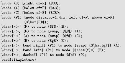
Figure 11.1 is a diagram drawn from raw TikZ code below:


FIGURE 11.1: A diagram drawn with TikZ: the source code is written into a *.tex file and compiled to PDF by ![]() .
.
To develop tikz graphics, the programs qtikz or ktikz can be helpful, since they provide a graphical user interface (an editor), which allows one to preview the results.
Graphviz (Ellson et al., 2002) is an open source and popular graph visualization software package (http://www.graphviz.org); it is powerful for drawing diagrams of abstract graphs and networks. Graphviz contains a few “filters,” such as dot, to draw directed graphs, and neato to draw undirected graphs. When engine = ’dot’, dot is used by default; to use other filters, we can set, e.g., engine.path = ’neato’.
Figure 11.2 is an example taken from the documentation of Graphviz.
We used fig.ext = ‘pdf’ here to produce a PDF graph file, and we can change it to other file formats like PNG as well.

FIGURE 11.2: A diagram drawn with dot in Graphviz (taken from the dot manual).

If you want to draw diagrams in HTML documents generated from R Markdown, you may consider the DiagrammeR package (https://github.com/rich-iannone/DiagrammeR), which is an HTML widget package that wraps a few JavaScript libraries (see Section 14.5.3 for more information about HTML widgets).
Highlight is a free and open source software package by Andre Simon (http://www.andre-simon.de) to do syntax highlighting for a large variety of languages, including C, PHP, and R, etc. It can write the output in either ![]() or HTML.
or HTML.
When the chunk option engine = ’highlight’, the highlight program is called to generate the highlighted code chunk. The chunk option engine.opts is a character string to pass additional arguments to Highlight, e.g., we can specify the input syntax via -S, and the type of output via -O.
The chunk below was taken from the previous awk example; it uses the chunk option engine.opts = ’-S awk -O latex’ to tell Highlight that the input syntax is awk, and the output type is ![]() , so that Highlight can produce appropriate
, so that Highlight can produce appropriate ![]() commands on keywords. It may be difficult to see the colors in the printed version of this book, but at least we can see the first line is italic (comments).
commands on keywords. It may be difficult to see the colors in the printed version of this book, but at least we can see the first line is italic (comments).

Note that Highlight generates commands like hlnum{} (for numbers) and hlstr{} (for strings) to mark up different tokens in the code. These commands are mostly consistent with knitr’s syntax highlighting commands, but there are a few exceptions, e.g., hlslc{} (for comments) produced by Highlight is not a part of knitr’s commands, so we need to define it in the ![]() preamble. Similarly, if the Highlight output is HTML, we need to define CSS styles for the class
preamble. Similarly, if the Highlight output is HTML, we need to define CSS styles for the class hl slc.
There are two more engines that are essentially for any language: cat and asis. The cat engine calls the function cat() to write the code chunk to a file, and the filename can be provided in the chunk option engine.opts = list(file = ?). The asis engine does nothing but just write the code chunk as-is in the output. However, it respects the chunk options eval and echo: if either of these options is FALSE, the code chunk will be hidden from the output, which can be useful when you want to dynamically control whether to show some content in the output.
For example, we can write the code chunk below to a file named styles.css through the cat engine:

The following code chunk will be included in the final output if the variable internal.only is TRUE (imagine you have a portion of the report content that you only want to show internally in your group):

In fact, there is a major flaw in the engines for interpreted languages introduced before: a new engine session is established for every single code chunk of this engine. This means all code chunks are independent in memory, and the variables created in previous chunks will not be available in latter chunks. The only exception is R code chunks: all of them are evaluated in the same R session. To address this issue, we need to open a persistent session for an engine, and keep on running code chunks in this session. For example, we can create a variable in a Python code chunk, and continue using it in the next Python chunk.
The runr package (Xie, 2013) is an attempt to solve this problem. Currently it has experimental support for Bash and Julia code, based on socket connections. The basic idea is like this (take the Julia engine as example):
1. Open a background Julia process that starts a socket server and keeps listening (the background process is detached from the current R session by system(’julia script.jl’, wait = FALSE));
2. R connects to the Julia socket server via socketConnection(open = ’w’), and writes the Julia code chunk to the server;
3. Julia receives the code, evaluates it, and writes the standard output (as plain text) to the socket;
4. R reads from the socket via socketConnection(open = ’r’), and writes the Julia output to the report just like R code chunk output;
5. Repeat steps 2–4 if the next Julia code chunk comes in, and Julia will quit if we send the code quit() to it.
In this way, the Julia session will be live until we explicitly shut it down from R, and all Julia code chunks will be evaluated in the same Julia session. The runr package is still at its early stage, and community contribution is welcome.