3 Baseband Signaling and Pulse Shaping

Figure 3.1a shows a simple block diagram of a communication system. The sequence of source bits {b_i} are grouped into sequential blocks (vectors) of m bits {b_i}, and each binary vector b_i is mapped to one of 2^m pulses, p(b_i; t), which is transmitted over the channel.

The transmitted signal as a function of time can be written as

s (t) = \sum_{i} p (b_{i}; t - i T) (3.1)

$s (t) = \sum_{i} p (b_{i}; t - i T) (3.1)$

Images

FIGURE 3.1 (a) Communication system model. The source bits are grouped into binary vectors, which are mapped to a sequence of pulse shapes. (b) Channel model consisting of a linear, time-invariant system (transfer function) followed by additive noise.

where 1/T is the rate at which each group of m bits, or pulses, is introduced to the channel. The information (bit) rate is therefore m/T.

The channel in Figure 3.1a can be a radio link, which may distort the input signal s(t) in a variety of ways. For example, it may introduce pulse dispersion (due to finite bandwidth) and multipath, as well as additive background noise. The output of the channel is denoted as x(t), which is processed by the receiver to determine estimates of the source bits. The receiver can be quite complicated; however, for the purpose of this discussion, it is sufficient to assume only that it contains a front-end filter and a sampler, as shown in Figure 3.1a. This assumption is valid for a wide variety of detection strategies. The purpose of the receiver filter is to remove noise outside of the transmitted frequency band and to compensate for the channel frequency response.

A commonly used channel model is shown in Figure 3.1b and consists of a linear, time-invariant filter, denoted as G(f), followed by additive noise n(t). The channel output is, therefore,

x (t) = [g (t) * s (t)] + n (t) (3.2)

$x (t) = [g (t) * s (t)] + n (t) (3.2)$

where g(t) is the channel impulse response associated with G(f), and the asterisk denotes convolution,

g (t) * s (t) = \int_{- \infty}^{\infty} g (t - τ) s (τ) d τ

$g (t) * s (t) = \int_{- \infty}^{\infty} g (t - τ) s (τ) d τ$

This channel model accounts for all linear, time-invariant channel impairments, such as finite bandwidth and time-invariant multipath. It does not account for time-varying impairments, such as rapid fading due to time-varying multipath. Nevertheless, this model can be considered valid over short time periods during which the multipath parameters remain constant.

In Figures 3.1a, and 3.1b, it is assumed that all signals are baseband signals, which means that the frequency content is centered around f = 0 (DC). The channel passband, therefore, partially coincides with the transmitted spectrum. In general, this condition requires that the transmitted signal be modulated by an appropriate carrier frequency and demodulated at the receiver. In that case, the model in Figures 3.1a, and 3.1b still applies; however, baseband-equivalent signals must be derived from their modulated (passband) counterparts. Baseband signaling and pulse shaping refers to the way in which a group of source bits is mapped to a baseband transmitted pulse.

As a simple example of baseband signaling, we can take m = 1 (map each source bit to a pulse), assign a 0 bit to a pulse p(t), and a 1 bit to the pulse –p(t). Perhaps the simplest example of a baseband pulse is the rectangular pulse given by p(t) = 1, 0 < t ≤ T, and p(t) = 0 elsewhere. In this case, we can write the transmitted signal as

s (t) = \sum_{i} A_{i} p (t - i T) (3.3)

$s (t) = \sum_{i} A_{i} p (t - i T) (3.3)$

where each symbol A_i takes on a value of +1 or –1, depending on the value of the ith bit, and 1/T is the symbol rate, namely, the rate at which the symbols A_i are introduced to the channel.

The preceding example is called binary pulse amplitude modulation (PAM), since the data symbols A_i are binary valued, and they amplitude modulate the transmitted pulse p(t). The information rate (bits per second) in this case is the same as the symbol rate 1/T. As a simple extension of this signaling technique, we can increase m and choose A_i from one of M = 2^m values to transmit at bit rate m/T. This is known as M-ary PAM. For example, letting m = 2, each pair of bits can be mapped to a pulse in the set {p(t), –p(t), 3p(t), –3p(t)}.

In general, the transmitted symbols {A_i}, the baseband pulse p(t), and channel impulse response g(t) can be complex valued. For example, each successive pair of bits might select a symbol from the set {1, –1, j, –j}, where $j = \sqrt{- 1}$ $j = \sqrt{- 1}$ . This is a consequence of considering the baseband equivalent of passband modulation. (That is, generating a transmitted spectrum which is centered around a carrier frequency f_c.) Here we are not concerned with the relation between the passband and baseband equivalent models and simply point out that the discussion and results in this chapter apply to complex-valued symbols and pulse shapes.

As an example of a signaling technique which is not PAM, let m = 1 and

\begin{array}{l} p (0; t) = {\begin{array}{l} \sqrt{2} \sin (2 π f_{1} t) & 0 < t < T \\ 0 & elsewhere \end{array} \\ p (1; t) = {\begin{array}{l} \sqrt{2} \sin (2 π f_{2} t) & 0 < t < T \\ 0 & elsewhere \end{array} \end{array} (3.4)

$\begin{array}{l} p (0; t) = {\begin{array}{l} \sqrt{2} \sin (2 π f_{1} t) & 0 < t < T \\ 0 & elsewhere \end{array} \\ p (1; t) = {\begin{array}{l} \sqrt{2} \sin (2 π f_{2} t) & 0 < t < T \\ 0 & elsewhere \end{array} \end{array} (3.4)$

where f₁ and f₂ ≠ f₁ are fixed frequencies selected so that f₁T and f₂T (number of cycles for each bit) are multiples of 1/2. These pulses are orthogonal, namely,

\int_{0}^{T} p (1; t) p (0; t) d t = 0

$\int_{0}^{T} p (1; t) p (0; t) d t = 0$

This choice of pulse shapes is called binary frequency-shift keying (FSK).

Another example of a set of orthogonal pulse shapes for m = 2 bits/T is shown in Figure 3.2. As these pulses may have as many as three transitions within a symbol period, the transmitted spectrum occupies roughly four times the transmitted spectrum of binary PAM with a rectangular pulse shape. The spectrum is, therefore, spread across a much larger band than the smallest required for reliable transmission, assuming a data rate of 2/T. This type of signaling is referred to as spread-spectrum. Spread-spectrum signals are more robust with respect to interference from other transmitted signals than are narrowband signals.^*

Images

FIGURE 3.2 Four orthogonal spread-spectrum pulse shapes.

3.2 Intersymbol Interference and the Nyquist Criterion

Consider the transmission of a PAM signal illustrated in Figure 3.3. The source bits {b_i} are mapped to a sequence of levels {A_i}, which modulate the transmitter pulse p(t). The channel input is, therefore, given by Equation 3.3 where p(t) is the impulse response of the transmitter pulse-shaping filter P(f) shown in Figure 3.3. The input to the transmitter filter P(f) is the modulated sequence of delta functions ∑_iA_iδ(t–iT). The channel is represented by the transfer function G(f) (plus noise), which has impulse response g(t), and the receiver filter has transfer function R(f) with associated impulse response r(t).

Let h(t) be the overall impulse response of the combined transmitter, channel, and receiver, which has transfer function H(f) = P(f)G(f)R(f). We can write h(t) = p(t)*g(t)*r(t). The output of the receiver filter is then

y (t) = \sum_{i} A_{i} h (t - i T) + \tilde{n} (t) (3.5)

$y (t) = \sum_{i} A_{i} h (t - i T) + \tilde{n} (t) (3.5)$

where ñ(t) = r(t)*n(t) is the output of the filter R(f) with input n(t). Assuming that samples are collected at the output of the filter R(f) at the symbol rate 1/T, we can write the kth sample of y(t) as

\begin{matrix} y (k T) = \sum_{i} A_{i} h (k T - i T) + \tilde{n} (k T) \\ = A_{k} h (0) + \sum_{i \neq k} A_{i} h (k T - i T) + \tilde{n} (k T) \end{matrix} (3.6)

$\begin{matrix} y (k T) = \sum_{i} A_{i} h (k T - i T) + \tilde{n} (k T) \\ = A_{k} h (0) + \sum_{i \neq k} A_{i} h (k T - i T) + \tilde{n} (k T) \end{matrix} (3.6)$

The first term on the right-hand side of Equation 3.6 is the kth transmitted symbol scaled by the system impulse response at t = 0. If this were the only term on the right side of Equation 3.6, we could obtain the source bits without error by scaling the received samples by 1/h(0). The second term on the right-hand side of Equation 3.6 is called intersymbol interference, which reflects the view that neighboring symbols interfere with the detection of each desired symbol.

One possible criterion for choosing the transmitter and receiver filters is to minimize intersymbol interference. Specifically, if we choose p(t) and r(t) so that

h (k T) = {\begin{matrix} \begin{array}{l} 1 \\ 0 \end{array} & \begin{array}{l} k = 0 \\ k \neq 0 \end{array} \end{matrix} (3.7)

$h (k T) = {\begin{matrix} \begin{array}{l} 1 \\ 0 \end{array} & \begin{array}{l} k = 0 \\ k \neq 0 \end{array} \end{matrix} (3.7)$

Images

FIGURE 3.3 Baseband model of a pulse amplitude modulation system.

*This example can also be viewed as coded binary PAM. Namely, each pair of two source bits are mapped to 4 coded bits, which are transmitted via binary PAM with a rectangular pulse.

then the kth received sample is

y (k T) = A_{k} + \tilde{n} (k T) (3.8)

$y (k T) = A_{k} + \tilde{n} (k T) (3.8)$

In this case, the intersymbol interference has been eliminated. This choice of p(t) and r(t) is called a zero-forcing solution, since it forces the intersymbol interference to zero. Depending on the type of detection scheme used, a zero-forcing solution may not be desirable. This is because the probability of error also depends on the noise intensity, which generally increases when intersymbol interference is suppressed. It is instructive, however, to examine the properties of the zero-forcing solution.

We now view Equation 3.7 in the frequency domain. Since h(t) has Fourier transform

H (f) = P (f) G (f) R (f) (3.9)

$H (f) = P (f) G (f) R (f) (3.9)$

where P(f) is the Fourier transform of p(t), the bandwidth of H(f) is limited by the bandwidth of the channel G(f). We will assume that G(f) = 0, |f| > W. The sampled impulse response h(kT) can, therefore, be written as the inverse Fourier transform

h (k T) = \int_{- W}^{W} H (f) e^{j 2 π f k T} d f

$h (k T) = \int_{- W}^{W} H (f) e^{j 2 π f k T} d f$

Through a series of manipulations, this integral can be rewritten as an inverse discrete Fourier transform,

h (k T) = T \int_{- 1 / (2 T)}^{1 / (2 T)} H_{eq} (e^{j 2 π f T}) e^{j 2 π f k T} d f (3.10a)

$h (k T) = T \int_{- 1 / (2 T)}^{1 / (2 T)} H_{eq} (e^{j 2 π f T}) e^{j 2 π f k T} d f (3.10a)$

where

\begin{matrix} H_{eq} (e^{j 2 π f T}) = \frac{1}{T} \sum_{k} H (f + \frac{k}{T}) \\ = \frac{1}{T} \sum_{k} P (f + \frac{k}{T}) G (f + \frac{k}{T}) R (f + \frac{k}{T}) \end{matrix} (3.10b)

$\begin{matrix} H_{eq} (e^{j 2 π f T}) = \frac{1}{T} \sum_{k} H (f + \frac{k}{T}) \\ = \frac{1}{T} \sum_{k} P (f + \frac{k}{T}) G (f + \frac{k}{T}) R (f + \frac{k}{T}) \end{matrix} (3.10b)$

This relation states that H_eq(z), z = e^j2πfT, is the discrete Fourier transform of the sequence {h_k}, where h_k = h(kT). Sampling the impulse response h(t) therefore changes the transfer function H(f) to the aliased frequency response H_eq(e^j2πfT). From Equations 3.10 and 3.6 we conclude that H_eq(z) is the transfer function that relates the sequence of input data symbols {A_i} to the sequence of received samples {y_i}, where y_i = y(iT), in the absence of noise. This is illustrated in Figure 3.4. For this reason, H_eq(z) is called the equivalent discrete-time transfer function for the overall system transfer function H(f).

Images

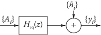
FIGURE 3.4 Equivalent discrete-time channel for the PAM system shown in Figure 3.3 [y_i = y(iT), ñ_i = ñ(iT)].

Since H_eq(e^j2πfT) is the discrete Fourier transform of the sequence {h_k}, the time-domain, or sequence condition (3.7) is equivalent to the frequency-domain condition

H_{eq} (e^{j 2 π f T}) = 1 (3.11)

$H_{eq} (e^{j 2 π f T}) = 1 (3.11)$

This relation is called the Nyquist criterion. From Equations 3.10b and 3.11 we make the following observations.

To satisfy the Nyquist criterion, the channel bandwidth W must be at least 1/(2T). Otherwise, G(f + n/T) = 0 for f in some interval of positive length for all n, which implies that H_eq(e^j2πfT) = 0 for f in the same interval.
For the minimum bandwidth W = 1/(2T), Equations 3.10b and 3.11 imply that H(f) = T for |f| < 1/(2T) and H(f) = 0 elsewhere. This implies that the system impulse response is given by

$h (t) = \frac{sin(π t / T)}{π t / T} (3.12)$ $h (t) = \frac{sin(π t / T)}{π t / T} (3.12)$

(Since $\int_{- \infty}^{\infty} h^{2} (t) d t = T,$ $\int_{- \infty}^{\infty} h^{2} (t) d t = T,$ the transmitted signal $S (t) = \sum_{i} A_{i} h (t - i T)$ $S (t) = \sum_{i} A_{i} h (t - i T)$ has power equal to the symbol variance E[|A_i|²].) The impulse response in Equation 3.12 is called a minimum bandwidth or Nyquist pulse. The frequency band [–1/(2T), 1/(2T)] [that is, the passband of H(f)] is called the Nyquist band.
Suppose that the channel is bandlimited to twice the Nyquist bandwidth. That is, G(f) = 0 for |f| > 1/T. The condition (3.11) then becomes

$H (f) + H (f - \frac{1}{T}) + H (f + \frac{1}{T}) = T (3.13)$ $H (f) + H (f - \frac{1}{T}) + H (f + \frac{1}{T}) = T (3.13)$

Assume for the moment that H(f) and h(t) are both real valued, so that H(f) is an even function of f [H(f) = H(–f)]. This is the case when the receiver filter is the matched filter (see Section 3.3). We can then rewrite Equation 3.13 as

$H (f) + H (\frac{1}{T} - f) = T, 0 < f < \frac{1}{2 T} (3.14)$ $H (f) + H (\frac{1}{T} - f) = T, 0 < f < \frac{1}{2 T} (3.14)$

which states that H(f) must have odd symmetry about f = 1/(2T). This is illustrated in Figure 3.5, which shows two different transfer functions H(f) that satisfy the Nyquist criterion.
The pulse shape p(t) enters into Equation 3.11 only through the product P(f)R(f). Consequently, either P(f) or R(f) can be fixed, and the other filter can be adjusted or adapted to the particular channel. Typically, the pulse shape p(t) is fixed, and the receiver filter is adapted to the (possibly time-varying) channel.

FIGURE 3.5 Two examples of frequency responses that satisfy the Nyquist criterion.

3.2.1 Raised Cosine Pulse

Suppose that the channel is ideal with transfer function

G (f) = {\begin{matrix} \begin{array}{l} 1, \\ 0, \end{array} & \begin{array}{l} | f | < W \\ | f | > W \end{array} \end{matrix} (3.15)

$G (f) = {\begin{matrix} \begin{array}{l} 1, \\ 0, \end{array} & \begin{array}{l} | f | < W \\ | f | > W \end{array} \end{matrix} (3.15)$

To maximize bandwidth efficiency, Nyquist pulses given by Equation 3.12 should be used where W = 1/(2T). This type of signaling, however, has two major drawbacks. First, Nyquist pulses are noncausal and of infinite duration. They can be approximated in practice by introducing an appropriate delay, and truncating the pulse. The pulse, however, decays very slowly, namely, as 1/t, so that the truncation window must be wide. This is equivalent to observing that the ideal bandlimited frequency response given by Equation 3.15 is difficult to approximate closely. The second drawback, which is more important, is the fact that this type of signaling is not robust with respect to sampling jitter. Namely, a small sampling offset ∊ produces the output sample

y (k T + ε) = \sum_{i} A_{i} \frac{\sin [π (k - i + ε / T)]}{π (k - i + ε / T)} (3.16)

$y (k T + ε) = \sum_{i} A_{i} \frac{\sin [π (k - i + ε / T)]}{π (k - i + ε / T)} (3.16)$

Since the Nyquist pulse decays as 1/t, this sum is not guaranteed to converge. A particular choice of symbols {A_i} can, therefore, lead to very large intersymbol interference, no matter how small the offset. Minimum bandwidth signaling is therefore impractical.

The preceding problem is generally solved in one of two ways in practice:

The pulse bandwidth is increased to provide a faster pulse decay than 1/t.
A controlled amount of intersymbol interference is introduced at the transmitter, which can be subtracted out at the receiver.

The former approach sacrifices bandwidth efficiency, whereas the latter approach sacrifices power efficiency. We will examine the latter approach in Section 3.5. The most common example of a pulse, which illustrates the first technique, is the raised cosine pulse, given by

h (t) = [\frac{\sin (π t / T)}{π t / T}] [\frac{\cos (α π t / T)}{1 - {(2 α t / T)}^{2}}] (3.17)

$h (t) = [\frac{\sin (π t / T)}{π t / T}] [\frac{\cos (α π t / T)}{1 - {(2 α t / T)}^{2}}] (3.17)$

which has Fourier transform

H (f) = {\begin{matrix} \begin{array}{l} T \\ \frac{T}{2} {1 + \cos [\frac{π T}{α} (| f | - \frac{1 - α}{2 T})]} \\ 0 \end{array} & \begin{array}{l} 0 \leq | f | \leq \frac{1 - α}{2 T} \\ \frac{1 - α}{2 T} \leq | f | \leq \frac{1 + α}{2 T} \\ | f | > \frac{1 + α}{2 T} \end{array} \end{matrix} (3.18)

$H (f) = {\begin{matrix} \begin{array}{l} T \\ \frac{T}{2} {1 + \cos [\frac{π T}{α} (| f | - \frac{1 - α}{2 T})]} \\ 0 \end{array} & \begin{array}{l} 0 \leq | f | \leq \frac{1 - α}{2 T} \\ \frac{1 - α}{2 T} \leq | f | \leq \frac{1 + α}{2 T} \\ | f | > \frac{1 + α}{2 T} \end{array} \end{matrix} (3.18)$

where 0 ≤ α ≤ 1.

Plots of p(t) and P(f) are shown in Figures 3.6a and 3.6b for different values of α. It is easily verified that h(t) satisfies the Nyquist criterion (3.7) and, consequently, H(f) satisfies Equation 3.11. When α = 0, H(f) is the Nyquist pulse with minimum bandwidth 1/(2T), and when α > 0, H(f) has bandwidth (1 + α)/(2T) with a raised cosine rolloff. The parameter α, therefore, represents the additional, or excess bandwidth as a fraction of the minimum bandwidth 1/(2T). For example, when α = 1, we say that the pulse is a raised cosine pulse with 100% excess bandwidth. This is because the pulse bandwidth 1/T is twice the minimum bandwidth. As the raised cosine pulse decays as 1/t³, performance is robust with respect to sampling offsets.

Images

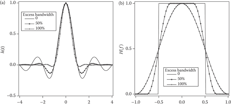
FIGURE 3.6 (a) Raised cosine pulse. (b) Raised cosine spectrum.

The raised cosine frequency response (3.18) applies to the combination of transmitter, channel, and receiver. If the transmitted pulse shape p(t) is a raised cosine pulse, then h(t) is a raised cosine pulse only if the combined receiver and channel frequency response is constant. Even with an ideal (transparent) channel, however, the optimum (matched) receiver filter response is generally not constant in the presence of additive Gaussian noise. An alternative is to transmit the square-root raised cosine pulse shape, which has frequency response P(f) given by the square-root of the raised cosine frequency response in Equation 3.18. Assuming an ideal channel, setting the receiver frequency response R(f) = P(f) then results in an overall raised cosine system response H(f).

3.3 Nyquist Criterion with Matched Filtering

Consider the transmission of an isolated pulse A₀δ(t). In this case the input to the receiver in Figure 3.3 is

x (t) = A_{0} \tilde{g} (t) + n (t) (3.19)

$x (t) = A_{0} \tilde{g} (t) + n (t) (3.19)$

where $\tilde{g} (t)$ $\tilde{g} (t)$ is the inverse Fourier transform of the combined transmitter-channel transfer function $\tilde{G} (f) = P (f) G (f)$ $\tilde{G} (f) = P (f) G (f)$ . We will assume that the noise n(t) is white with spectrum N₀/2. The output of the receiver filter is then

y (t) = r (t) * x (t) = A_{0} [r (t) * \tilde{g} (t)] + [r (t) * n (t)] (3.20)

$y (t) = r (t) * x (t) = A_{0} [r (t) * \tilde{g} (t)] + [r (t) * n (t)] (3.20)$

The first term on the right-hand side is the desired signal, and the second term is noise. Assuming that y(t) is sampled at t = 0, the ratio of signal energy to noise energy, or signal-to-noise ratio (SNR) at the sampling instant, is

S N R = \frac{E [{| A_{0} |}^{2}] {| \int_{- \infty}^{\infty} r (- t) \tilde{g} (t) d t |}^{2}}{\frac{N_{0}}{2} \int_{- \infty}^{\infty} {| r (t) |}^{2} d t} (3.21)

$S N R = \frac{E [{| A_{0} |}^{2}] {| \int_{- \infty}^{\infty} r (- t) \tilde{g} (t) d t |}^{2}}{\frac{N_{0}}{2} \int_{- \infty}^{\infty} {| r (t) |}^{2} d t} (3.21)$

The receiver impulse response that maximizes this expression is $r (t) = {\tilde{g}}^{*} (- t)$ $r (t) = {\tilde{g}}^{*} (- t)$ [complex conjugate of $\tilde{g} (- t)$ $\tilde{g} (- t)$ ], which is known as the matched filter impulse response. The associated transfer function is $R (f) = {\tilde{G}}^{*} (f)$ $R (f) = {\tilde{G}}^{*} (f)$ .

Choosing the receiver filter to be the matched filter is optimal in more general situations, such as when detecting a sequence of channel symbols with intersymbol interference (assuming the additive noise is Gaussian). We, therefore, reconsider the Nyquist criterion when the receiver filter is the matched filter. In this case, the baseband model is shown in Figure 3.7, and the output of the receiver filter is given by

y (t) = \sum_{i} A_{i} h (t - i T) + \tilde{n} (t) (3.22)

$y (t) = \sum_{i} A_{i} h (t - i T) + \tilde{n} (t) (3.22)$

where the baseband pulse h(t) is now the impulse response of the filter with transfer function $| \tilde{G} (f) |^{2} = | P (f) G (f) |^{2}$ $| \tilde{G} (f) |^{2} = | P (f) G (f) |^{2}$ . This impulse response is the autocorrelation of the impulse response of the combined transmitter-channel filter $\tilde{G} (f)$ $\tilde{G} (f)$ ,

h (t) = \int_{- \infty}^{\infty} {\tilde{g}}^{*} (s) \tilde{g} (s + t) d s (3.23)

$h (t) = \int_{- \infty}^{\infty} {\tilde{g}}^{*} (s) \tilde{g} (s + t) d s (3.23)$

With a matched filter at the receiver, the equivalent discrete-time transfer function is

\begin{matrix} H_{eq} (e^{j 2 π f T}) = \frac{1}{T} {\sum_{k} | \tilde{G} (f - \frac{k}{T}) |}^{2} \\ = \frac{1}{T} {\sum_{k} | P (f - \frac{k}{T}) G (f - \frac{k}{T}) |}^{2} \end{matrix} (3.24)

$\begin{matrix} H_{eq} (e^{j 2 π f T}) = \frac{1}{T} {\sum_{k} | \tilde{G} (f - \frac{k}{T}) |}^{2} \\ = \frac{1}{T} {\sum_{k} | P (f - \frac{k}{T}) G (f - \frac{k}{T}) |}^{2} \end{matrix} (3.24)$

which relates the sequence of transmitted symbols {A_k} to the sequence of received samples {y_k} in the absence of noise. Note that H_eq(e^j2πfT) is positive, real valued, and an even function of f. If the channel is bandlimited to twice the Nyquist bandwidth, then H(f) = 0 for |f| > 1/T, and the Nyquist condition is given by Equation 3.14 where H(f) = |G(f)P(f)|². The aliasing sum in Equation 3.10b can therefore be described as a folding operation in which the channel response |H(f)|² is folded around the Nyquist frequency 1/(2T). For this reason, H_eq(e^j2πfT) with a matched receiver filter is often referred to as the folded channel spectrum.

Images

FIGURE 3.7 Baseband PAM model with a matched filter at the receiver.

3.4 Eye Diagrams

One way to assess the severity of distortion due to intersymbol interference in a digital communications system is to examine the eye diagram. The eye diagram is illustrated in Figures 3.8a and 3.8b, for a raised cosine pulse shape with 25% excess bandwidth and an ideal bandlimited channel. Figure 3.8a shows the data signal at the receiver

y (t) = \sum_{i} A_{i} h (t - i T) + \tilde{n} (t) (3.25)

$y (t) = \sum_{i} A_{i} h (t - i T) + \tilde{n} (t) (3.25)$

where h(t) is given by Equation 3.17, α = 1/4, each symbol A_i is independently chosen from the set {±1, ±3}, where each symbol is equally likely, and ñ(t) is bandlimited white Gaussian noise. (The received SNR is 30 dB.) The eye diagram is constructed from the time-domain data signal y(t) as follows (assuming nominal sampling times at kT, k = 0, 1, 2, …):

Partition the waveform y(t) into successive segments of length T starting from t = T/2.
Translate each of these waveform segments [y(t), (k + 1/2)T ≤ t ≤ (k + 3/2)T, k = 0, 1, 2, …] to the interval [–T/2, T/2], and superimpose.

The resulting picture is shown in Figure 3.8b for the y(t) shown in Figure 3.8a. (Partitioning y(t) into successive segments of length iT, i > 1, is also possible. This would result in i successive eye diagrams.) The number of eye openings is one less than the number of transmitted signal levels. In practice, the eye diagram is easily viewed on an oscilloscope by applying the received waveform y(t) to the vertical deflection plates of the oscilloscope and applying a sawtooth waveform at the symbol rate 1/T to the horizontal deflection plates. This causes successive symbol intervals to be translated into one interval on the oscilloscope display.

Each waveform segment y(t), (k + 1/2)T ≤ t ≤ (k + 3/2)T, depends on the particular sequence of channel symbols surrounding A_k. The number of channel symbols that affects a particular waveform segment depends on the extent of the intersymbol interference, shown in Equation 3.6. This, in turn, depends on the duration of the impulse response h(t). For example, if h(t) has most of its energy in the interval 0 < t < mT, then each waveform segment depends on approximately m symbols. Assuming binary transmission, this implies that there are a total of 2^m waveform segments that can be superimposed in the eye diagram. (It is possible that only one sequence of channel symbols causes significant intersymbol interference, and this sequence occurs with very low probability.) In current digital wireless applications the impulse response typically spans only a few symbols.

Images

FIGURE 3.8 (a) Received signal y(t). (b) Eye diagram for received signal shown in Figure 3.8a.

The eye diagram has the following important features which measure the performance of a digital communications system.

3.4.1 Vertical Eye Opening

The vertical openings at any time t₀, –T/2 ≤ t₀ ≤ T/2, represent the separation between signal levels with worst-case intersymbol interference, assuming that y(t) is sampled at times t = kT + t₀, k = 0, 1, 2, …. It is possible for the intersymbol interference to be large enough so that this vertical opening between some, or all, signal levels disappears altogether. In that case, the eye is said to be closed. Otherwise, the eye is said to be open. A closed eye implies that if the estimated bits are obtained by thresholding the samples y(kT), then the decisions will depend primarily on the intersymbol interference rather than on the desired symbol. The probability of error will, therefore, be close to 1/2. Conversely, wide vertical spacings between signal levels imply a large degree of immunity to additive noise. In general, y(t) should be sampled at the times kT + t₀, k = 0, 1, 2, …, where t₀ is chosen to maximize the vertical eye opening.

3.4.2 Horizontal Eye Opening

The width of each opening indicates the sensitivity to timing offset. Specifically, a very narrow eye opening indicates that a small timing offset will result in sampling where the eye is closed. Conversely, a wide horizontal opening indicates that a large timing offset can be tolerated, although the error probability will depend on the vertical opening.

3.4.3 Slope of the Inner Eye

The slope of the inner eye indicates sensitivity to timing jitter or variance in the timing offset. Specifically, a very steep slope means that the eye closes rapidly as the timing offset increases. In this case, a significant amount of jitter in the sampling times significantly increases the probability of error.

The shape of the eye diagram is determined by the pulse shape. In general, the faster the baseband pulse decays, the wider the eye opening. For example, a rectangular pulse produces a box-shaped eye diagram (assuming binary signaling). The minimum bandwidth pulse shape Equation 3.12 produces an eye diagram which is closed for all t except for t = 0. This is because, as shown earlier, an arbitrarily small timing offset can lead to an intersymbol interference term that is arbitrarily large, depending on the data sequence.

3.5 Partial-Response Signaling

To avoid the problems associated with Nyquist signaling over an ideal bandlimited channel, bandwidth and/or power efficiency must be compromised. Raised cosine pulses compromise bandwidth efficiency to gain robustness with respect to timing errors. Another possibility is to introduce a controlled amount of intersymbol interference at the transmitter, which can be removed at the receiver. This approach is called partial-response (PR) signaling. The terminology reflects the fact that the sampled system impulse response does not have the full response given by the Nyquist condition Equation 3.7.

To illustrate PR signaling, suppose that the Nyquist condition Equation 3.7 is replaced by the condition

h_{k} = {\begin{array}{l} 1 & k = 0, 1 \\ 0 & all other k \end{array} (3.26)

$h_{k} = {\begin{array}{l} 1 & k = 0, 1 \\ 0 & all other k \end{array} (3.26)$

The kth received sample is then

y_{k} = A_{k} + A_{k - 1} + {\tilde{n}}_{k} (3.27)

$y_{k} = A_{k} + A_{k - 1} + {\tilde{n}}_{k} (3.27)$

so that there is intersymbol interference from one neighboring transmitted symbol. For now we focus on the spectral characteristics of PR signaling and defer discussion of how to detect the transmitted sequence {A_k} in the presence of intersymbol interference. The equivalent discrete-time transfer function in this case is the discrete Fourier transform of the sequence in Equation 3.26,

\begin{matrix} H_{eq} (e^{j 2 π f T}) = \frac{1}{T} \sum_{k} H (f + \frac{k}{T}) \\ = 1 + e^{- j 2 π f T} = 2 e^{- j π f T} \cos (π f T) \end{matrix} (3.28)

$\begin{matrix} H_{eq} (e^{j 2 π f T}) = \frac{1}{T} \sum_{k} H (f + \frac{k}{T}) \\ = 1 + e^{- j 2 π f T} = 2 e^{- j π f T} \cos (π f T) \end{matrix} (3.28)$

As in the full-response case, for Equation 3.28 to be satisfied, the minimum bandwidth of the channel G(f) and transmitter filter P(f) is W = 1/(2T). Assuming P(f) has this minimum bandwidth implies

H (f) = {\begin{array}{l} 2 T e^{- j π f T} \cos (π f T) & | f | < 1 / (2 T) \\ 0 & | f | > 1 / (2 T) \end{array} (3.29a)

$H (f) = {\begin{array}{l} 2 T e^{- j π f T} \cos (π f T) & | f | < 1 / (2 T) \\ 0 & | f | > 1 / (2 T) \end{array} (3.29a)$

and

h (t) = T {sinc (t / T) + sinc [(t - T) / T]} (3.29b)

$h (t) = T {sinc (t / T) + sinc [(t - T) / T]} (3.29b)$

where sinc x = (sin πx)/(πx). This pulse is called a duobinary pulse and is shown along with the associated H(f) in Figure 3.9. [Notice that h(t) satisfies Equation 3.26.] Unlike the ideal bandlimited frequency response, the transfer function H(f) in Equation 3.29a is continuous and is, therefore, easily approximated by a physically realizable filter. Duobinary PR was first proposed by Lender, [1], and later generalized by Kretzmer, [2].

The main advantage of the duobinary pulse Equation 3.29b, relative to the minimum bandwidth pulse Equation 3.12, is that signaling at the Nyquist symbol rate is feasible with zero excess bandwidth. As the pulse decays much more rapidly than a Nyquist pulse, it is robust with respect to timing errors. Selecting the transmitter and receiver filters so that the overall system response is duobinary is appropriate in situations where the channel frequency response G(f) is near zero or has a rapid rolloff at the Nyquist band edge f = 1/(2T).

Images

FIGURE 3.9 Duobinary frequency response and minimum bandwidth pulse.

As another example of PR signaling, consider the modified duobinary partial response

h_{k} = {\begin{array}{l} 1 & k = - 1 \\ - 1 & k = 1 \\ 0 & all other k \end{array} (3.30)

$h_{k} = {\begin{array}{l} 1 & k = - 1 \\ - 1 & k = 1 \\ 0 & all other k \end{array} (3.30)$

which has an equivalent discrete-time transfer function

\begin{matrix} H_{eq} (e^{j 2 π f T}) = e^{j 2 π f T} - e^{- j 2 π f T} \\ = j 2 \sin (2 π f T) \end{matrix} (3.31)

$\begin{matrix} H_{eq} (e^{j 2 π f T}) = e^{j 2 π f T} - e^{- j 2 π f T} \\ = j 2 \sin (2 π f T) \end{matrix} (3.31)$

With zero excess bandwidth, the overall system response is

H (f) = {\begin{array}{l} j 2 T \sin (2 π f T) & | f | < 1 / (2 T) \\ 0 & | f | > 1 / (2 T) \end{array} (3.32a)

$H (f) = {\begin{array}{l} j 2 T \sin (2 π f T) & | f | < 1 / (2 T) \\ 0 & | f | > 1 / (2 T) \end{array} (3.32a)$

and

h (t) = T {sinc [(t + T) / T] - sinc [(t - T)/ T]} (3.32b)

$h (t) = T {sinc [(t + T) / T] - sinc [(t - T)/ T]} (3.32b)$

These functions are plotted in Figure 3.10. This pulse shape is appropriate when the channel response G(f) is near zero at both DC (f = 0) and at the Nyquist band edge. This is often the case for wire (twisted-pair) channels where the transmitted signal is coupled to the channel through a transformer. Like duobinary PR, modified duobinary allows minimum bandwidth signaling at the Nyquist rate.

Images

FIGURE 3.10 Modified duobinary frequency response and minimum bandwidth pulse.

Images

FIGURE 3.11 Generation of PR signal.

A particular partial response is often identified by the polynomial

\sum_{k = 0}^{K} h_{k} D^{k}

$\sum_{k = 0}^{K} h_{k} D^{k}$

where D (for delay) takes the place of the usual z⁻¹ in the z transform of the sequence {h_k}. For example, duobinary is also referred to as 1 + D partial response.

In general, more complicated system responses than those shown in Figures 3.9 and 3.10 can be generated by choosing more nonzero coefficients in the sequence {h_k}. This complicates detection, however, because of the additional intersymbol interference that is generated.

Rather than modulating a PR pulse h(t), a PR signal can also be generated by filtering the sequence of transmitted levels {A_i}. This is shown in Figure 3.11. Namely, the transmitted levels are first passed through a discrete-time (digital) filter with transfer function P_d(e^j2πfT) (where the subscript d indicates discrete). [Note that P_d(e^j2πfT) can be selected to be H_eq(e^j2πfT).] The outputs of this filter form the PAM signal, where the pulse shaping filter P(f) = 1, |f| < 1/(2T) and is zero elsewhere. If the transmitted levels {A_k} are selected independently and are identically distributed, then the transmitted spectrum is $σ_{A}^{2} | P_{d} (e^{j 2 π f T}) |^{2}$ $σ_{A}^{2} | P_{d} (e^{j 2 π f T}) |^{2}$ for |f| < 1/(2T) and is zero for |f| > 1/(2T), where $σ_{A}^{2} = E [| A_{k} |^{2}]$ $σ_{A}^{2} = E [| A_{k} |^{2}]$ .

Shaping the transmitted spectrum to have nulls coincident with nulls in the channel response potentially offers significant performance advantages. By introducing intersymbol interference, however, PR signaling increases the number of received signal levels, which increases the complexity of the detector and may reduce immunity to noise. For example, the set of received signal levels for duobinary signaling is {0, ±2} from which the transmitted levels {±1} must be estimated. The performance of a particular PR scheme depends on the channel characteristics, as well as the type of detector used at the receiver. We now describe a simple suboptimal detection strategy.

3.5.1 Precoding

Consider the received signal sample Equation 3.27 with duobinary signaling. If the receiver has correctly decoded the symbol A_k₋₁, then in the absence of noise A_k can be decoded by subtracting A_k₋₁ from the received sample y_k. If an error occurs, however, then subtracting the preceding symbol estimate from the received sample will cause the error to propagate to successive detected symbols. To avoid this problem, the transmitted levels can be precoded in such a way as to compensate for the intersymbol interference introduced by the overall partial response.

We first illustrate precoding for duobinary PR. The sequence of operations is illustrated in Figure 3.12. Let {b_k} denote the sequence of source bits where b_k ∈ {0, 1}. This sequence is transformed to the sequence ${{b^{'}}_{k}}$ ${{b^{'}}_{k}}$ by the operation

{b^{'}}_{k} = b_{k} \oplus {b^{'}}_{k - 1} (3.33)

${b^{'}}_{k} = b_{k} \oplus {b^{'}}_{k - 1} (3.33)$

Images

FIGURE 3.12 Precoding for a PR channel.

where ⊕ denotes modulo 2 addition (exclusive OR). The sequence ${{b^{'}}_{k}}$ ${{b^{'}}_{k}}$ is mapped to the sequence of binary transmitted signal levels {A_k} according to

A_{k} = 2 {b^{'}}_{k} - 1 (3.34)

$A_{k} = 2 {b^{'}}_{k} - 1 (3.34)$

That is, ${b^{'}}_{k} = 0 ({b^{'}}_{k} = 1)$ ${b^{'}}_{k} = 0 ({b^{'}}_{k} = 1)$ is mapped to the transmitted level A_k = –1 (A_k = 1). In the absence of noise, the received symbol is then

y_{k} = A_{k} + A_{k - 1} = 2 ({b^{'}}_{k} + {b^{'}}_{k - 1} - 1) (3.35)

$y_{k} = A_{k} + A_{k - 1} = 2 ({b^{'}}_{k} + {b^{'}}_{k - 1} - 1) (3.35)$

and combining Equations 3.33 and 3.35 gives

b_{k} = (\frac{1}{2} y_{k} + 1) \mod 2 (3.36)

$b_{k} = (\frac{1}{2} y_{k} + 1) \mod 2 (3.36)$

That is, if y_k = ±2, then b_k = 0, and if y_k = 0, then b_k = 1. Precoding, therefore, enables the detector to make symbol-by-symbol decisions that do not depend on previous decisions. Table 3.1 shows a sequence of transmitted bits {b_i}, precoded bits ${{b^{'}}_{i}}$ ${{b^{'}}_{i}}$ , transmitted signal levels {A_i}, and received samples {y_i}.

The preceding precoding technique can be extended to multilevel PAM and to other PR channels. Suppose that the PR is specified by

H_{eq} (D) = \sum_{k = 0}^{K} h_{k} D^{k}

$H_{eq} (D) = \sum_{k = 0}^{K} h_{k} D^{k}$

where the coefficients are integers and that the source symbols {b_k} are selected from the set {0, 1, …, M–1}. These symbols are transformed to the sequence ${{b^{'}}_{k}}$ ${{b^{'}}_{k}}$ via the precoding operation

{b^{'}}_{k} = (b_{k} - \sum_{i = 1}^{K} h_{i} {b^{'}}_{k - i}) \mod M (3.37)

${b^{'}}_{k} = (b_{k} - \sum_{i = 1}^{K} h_{i} {b^{'}}_{k - i}) \mod M (3.37)$

Because of the modulo operation, each symbol ${b^{'}}_{k}$ ${b^{'}}_{k}$ is also in the set {0, 1, …, M–1}. The kth transmitted signal level is given by

A_{k} = 2 {b^{'}}_{k} - (M - 1) (3.38)

$A_{k} = 2 {b^{'}}_{k} - (M - 1) (3.38)$

so that the set of transmitted levels is {–(M – 1), …, (M – 1)} (i.e., a shifted version of the set of values assumed by b_k). In the absence of noise the received sample is

y_{k} = \sum_{i = 0}^{K} h_{i} A_{k - i} (3.39)

$y_{k} = \sum_{i = 0}^{K} h_{i} A_{k - i} (3.39)$

TABLE 3.1 Example of Precoding for Duobinary PR

Images

and it can be shown that the kth source symbol is given by

b_{k} = \frac{1}{2} (y_{k} + (M - 1) \cdot H_{eq} (1)) \mod M (3.40)

$b_{k} = \frac{1}{2} (y_{k} + (M - 1) \cdot H_{eq} (1)) \mod M (3.40)$

Precoding the symbols {b_k} in this manner, therefore, enables symbol-by-symbol decisions at the receiver. In the presence of noise, more sophisticated detection schemes (e.g., maximum likelihood) can be used with PR signaling to obtain improvements in performance.

3.6 Additional Considerations

In many applications, bandwidth and intersymbol interference are not the only important considerations for selecting baseband pulses. Here we give a brief discussion on additional practical constraints that may influence this selection.

3.6.1 Average Transmitted Power and Spectral Constraints

The constraint on average transmitted power varies according to the application. For example, low-average power is highly desirable for mobile wireless applications that use battery-powered transmitters. In many applications (e.g., digital subscriber loops, as well as digital radio), constraints are imposed to limit the amount of interference, or crosstalk, radiated into neighboring receivers and communications systems. Because this type of interference is frequency dependent, the constraint may take the form of a spectral mask that specifies the maximum allowable transmitted power as a function of frequency. For example, crosstalk in wireline channels is generally caused by capacitive coupling and increases as a function of frequency. Consequently, to reduce the amount of crosstalk generated at a particular transmitter, the pulse shaping filter generally attenuates high frequencies more than low frequencies.

In radio applications where signals are assigned different frequency bands, constraints on the transmitted spectrum are imposed to limit adjacent-channel interference. This interference is generated by transmitters assigned to adjacent frequency bands. Therefore, a constraint is needed to limit the amount of out-of-band power generated by each transmitter, in addition to an overall average power constraint. To meet this constraint, the transmitter filter in Figure 3.3 must have a sufficiently steep rolloff at the edges of the assigned frequency band. (Conversely, if the transmitted signals are time multiplexed, then the duration of the system impulse response must be contained within the assigned time slot.)

3.6.2 Peak-to-Average Power

In addition to a constraint on average transmitted power, a peak-power constraint is often imposed as well. This constraint is important in practice for the following reasons:

The dynamic range of the transmitter is limited. In particular, saturation of the output amplifier will “clip” the transmitted waveform.
Rapid fades can severely distort signals with high peak-to-average power.
The transmitted signal may be subjected to nonlinearities. Saturation of the output amplifier is one example. Another example that pertains to wireline applications is the companding process in the voice telephone network [3]. Namely, the compander used to reduce quantization noise for pulse-code modulated voice signals introduces amplitude-dependent distortion in data signals.

The preceding impairments or constraints indicate that the transmitted waveform should have a low peak-to-average power ratio (PAR). For a transmitted waveform x(t), the PAR is defined as

PAR = \frac{max {| x (t) |}^{2}}{E {{| x (t) |}^{2}}}

$PAR = \frac{max {| x (t) |}^{2}}{E {{| x (t) |}^{2}}}$

where E(·) denotes expectation. Using binary signaling with rectangular pulse shapes minimizes the PAR. However, this compromises bandwidth efficiency. In applications where PAR should be low, binary signaling with rounded pulses is often used. Operating RF power amplifiers with power back-off can also reduce PAR, but leads to inefficient amplification.

For an orthogonal frequency division multiplexing (OFDM) system, it is well known that the transmitted signal can exhibit a very high PAR compared to an equivalent single-carrier system. Hence more sophisticated approaches to PAR reduction are required for OFDM. Some proposed approaches are described in Reference 4 and references therein. These include altering the set of transmitted symbols and setting aside certain OFDM tones specifically to minimize PAR.

3.6.3 Channel and Receiver Characteristics

The type of channel impairments encountered and the type of detection scheme used at the receiver can also influence the choice of a transmitted pulse shape. For example, a constant amplitude pulse is appropriate for a fast fading environment with noncoherent detection. The ability to track channel characteristics, such as phase, may allow more bandwidth efficient pulse shapes in addition to multilevel signaling.

High-speed data communications over time-varying channels requires that the transmitter and/or receiver adapt to the changing channel characteristics. Adapting the transmitter to compensate for a time-varying channel requires a feedback channel through which the receiver can notify the transmitter of changes in channel characteristics. Because of this extra complication, adapting the receiver is often preferred to adapting the transmitter pulse shape. However, the following examples are notable exceptions.

Mobile cellular systems may dynamically adapt the transmitter power for each link (in both directions) to control the amount of interference generated and to compensate for channel conditions. This can be viewed as a simple form of adaptive transmitter pulse shaping in which a single parameter associated with the pulse shape is varied.
Multitone modulation divides the channel bandwidth into small subbands, and the transmitted power and source bits are distributed among these subbands to maximize the information rate. The received signal-to-noise ratio for each subband must be transmitted back to the transmitter to guide the allocation of transmitted bits and power [5].

In addition to multitone modulation, adaptive precoding (also known as Tomlinson–Harashima precoding [6,7]) is another way in which the transmitter can adapt to the channel frequency response. Adaptive precoding is an extension of the technique described earlier for partial-response channels. Namely, the equivalent discrete-time channel impulse response is measured at the receiver and sent back to the transmitter, where it is used in a precoder. The precoder compensates for the intersymbol interference introduced by the channel, allowing the receiver to detect the data by a simple threshhold operation. Both multitone modulation and precoding have been used with wireline channels (voiceband modems and digital subscriber loops).

3.6.4 Complexity

Generation of a bandwidth-efficient signal requires a filter with a sharp cutoff. In addition, bandwidth-efficient pulse shapes can complicate other system functions, such as timing and carrier recovery. If sufficient bandwidth is available, the cost can be reduced by using a rectangular pulse shape with a simple detection strategy (low-pass filter and threshold).

3.6.5 Tolerance to Interference

Interference is one of the primary channel impairments associated with digital radio. In addition to adjacent-channel interference described earlier, cochannel interference may be generated by other transmitters assigned to the same frequency band as the desired signal. Cochannel interference can be controlled through frequency (and perhaps time slot) assignments and by pulse shaping. For example, assuming fixed average power, increasing the bandwidth occupied by the signal lowers the power spectral density and decreases the amount of interference into a narrowband system that occupies part of the available bandwidth. Sufficient bandwidth spreading, therefore, enables wideband signals to be overlaid on top of narrowband signals without disrupting either service.

3.6.6 Privacy and Security

The broadcast nature of wireless channels generally makes eavesdropping easier than for wired channels. A requirement for most commercial, as well as military applications, is to guarantee the privacy of user conversations (low probability of intercept). An additional requirement, in some applications, is that determining whether or not communications is taking place must be difficult (low probability of detection). Spread-spectrum waveforms are attractive in these applications since spreading the pulse energy over a wide frequency band decreases the power spectral density, and hence makes the signal less visible. Power-efficient modulation combined with coding enables a further reduction in transmitted power for a target error rate.

3.7 Examples

We conclude this chapter with a brief description of baseband pulse shapes used in existing standards for digital mobile cellular systems.

3.7.1 Wideband Code Division Multiple Access (W-CDMA)

W-CDMA refers to the radio transmission part of Universal Mobile Telecommunications System (UMTS), which is an evolution from the European GSM standard developed by the Third Generation Partnership Project (3GPP) [8]. It operates in both frequency-division duplex (FDD) and time-division duplex (TDD) modes as part of UMTS Terrestrial Radio Access (UTRA). The transmit pulse-shaping filter for W-CDMA is a square-root raised cosine pulse with roll-off factor α = 0.22. The chip impulse response is given by

p (t) = \frac{\sin (π \frac{t}{T_{C}} (1 - α)) + 4 α \frac{t}{T_{C}} \cos (π \frac{t}{T_{C}} (1 + α))}{π \frac{t}{T_{C}} (1 - {(4 α \frac{t}{T_{C}})}^{2})}

$p (t) = \frac{\sin (π \frac{t}{T_{C}} (1 - α)) + 4 α \frac{t}{T_{C}} \cos (π \frac{t}{T_{C}} (1 + α))}{π \frac{t}{T_{C}} (1 - {(4 α \frac{t}{T_{C}})}^{2})}$

where the chip duration T_c = (1/chiprate) = 0.24414 µs.

3.7.2 CDMA2000

CDMA2000 is an evolution from the North American Interim Standard-95 (IS-95) developed by the Third Generation Partnership Project 2 (3GPP2). The 3GPP2 standard has defined baseband filters for CDMA2000 for the In-phase (I-channel) and Quadrature-phase (Q-channel) signals prior to modulation [9]. These baseband filters have a normalized frequency response given by

S (f) = {\begin{array}{l} \pm δ_{1}, & in the passband 0 ≪ f ≪ f_{p} \\ - δ_{2}, & in the shopband f ≫ f_{s} \end{array}

$S (f) = {\begin{array}{l} \pm δ_{1}, & in the passband 0 ≪ f ≪ f_{p} \\ - δ_{2}, & in the shopband f ≫ f_{s} \end{array}$

where δ₁ = 1.5 dB, δ₂ = 40 dB, f_p = 590 kHz, and f_s = 740 kHz. The impulse response s(t) of the baseband filter is given by a scaled and delayed version of the coefficients h(k) in Table 2.1.3.1.13.1-1 in Reference 9. Specifically, a scale factor κ and delay τ are selected to minimize the mean squared error

M S E = \sum_{k = 0}^{\infty} {[κ s (k T_{s} - τ) - h (k)]}^{2}

$M S E = \sum_{k = 0}^{\infty} {[κ s (k T_{s} - τ) - h (k)]}^{2}$

where T_s = 203.451 ns is one quarter of the duration of the CDMA2000 chip.

3.7.3 Wireless Local Area Networks (WLAN)

The IEEE 802.11 working group has developed requirements for the spectral mask for WLANs in Sections 17.3.9.2 and 17.3.9.6 of Reference 10.^* Any combination of time-domain windowing and frequency-domain filtering methods may be used to achieve those objectives. IEEE 802.11 has provided informative parameters for a time-domain windowing method that may be used to filter the I- and Q-channel signals prior to modulation. The time-windowing function is given by [10]:

w_{T} (t) = {\begin{array}{l} \sin^{2} (\frac{π}{2} (0.5 T + t / T_{T R})), for - T_{T R} / 2 < t < T_{T R} / 2 \\ 1, for T_{T R} / 2 \leq t < T - T_{T R} / 2 \\ \sin^{2} (\frac{π}{2} (0.5 T - (t - T) / T_{T R})), for T - T_{T R} / 2 \leq t < T + T_{T R} / 2 \end{array}

$w_{T} (t) = {\begin{array}{l} \sin^{2} (\frac{π}{2} (0.5 T + t / T_{T R})), for - T_{T R} / 2 < t < T_{T R} / 2 \\ 1, for T_{T R} / 2 \leq t < T - T_{T R} / 2 \\ \sin^{2} (\frac{π}{2} (0.5 T - (t - T) / T_{T R})), for T - T_{T R} / 2 \leq t < T + T_{T R} / 2 \end{array}$

where T_TR (approximately 100 ns) is selected to smooth transitions between consecutive OFDM symbols. This creates a small overlap between the consecutive symbols. Smoothing this transition reduces the spectral sidelobes of the transmitted waveform. In the case of vanishing T_TR, the windowing function degenerates to a rectangular pulse of duration T.

3.7.4 Worldwide Interoperability for Microwave Access (WiMAX)

WiMAX is a broadband wireless access technology, and refers to the IEEE 802.16 standard [11]. The 802.16 air interface is based on OFDM, and has specified a square-root raised cosine filter with excess bandwidth factor α = 0.25 for the I- and Q-channels prior to modulation. The filter transfer function is therefore the square root of H(f) in Equation 3.18, where T is the OFDM symbol period.

*Reference 10 was created by merging 802.11a, b, d, e, g, h, i, and j amendments with the base 802.11 standard and renamed to the current base standard IEEE 802.11-2007. (The high-throughput amendment 802.11n also references this windowing function.)

3.7.5 Long-Term Evolution (LTE)

LTE is an evolution of UMTS, defined in the 3GPP Release 8 specification. Evolved UTRA (E-UTRA) is the air interface for LTE, which operates in both FDD and TDD modes, as well as half-duplex FDD with the same radio access technology. LTE uses Orthogonal Frequency Division Multiple Access (OFDMA) radio-access for the downlink and Single-Carrier Frequency Division Multiple Access (SC-FDMA) on the uplink. Unlike UTRA, which uses a square-root raised cosine pulse shaping filter, E-UTRA uses a rectangular transmit pulse shaping filter [12].

References

1. Lender, A., The duobinary technique for high-speed data Transmission. AIEE Trans. on Comm. Electronics, 82 (March), 214–218, 1963.

2. Kretzmer, E. R., Generalization of a technique for binary data communication. IEEE Trans. Comm. Tech., COM-14(Feb.), 67, 68, 1966.

3. Kalet, I. and Saltzberg, B. R., QAM transmission through a companding channel—Signal constellations and detection. IEEE Trans. on Comm., 42(2–4), 417–429, 1994.

4. Muller, S. H. and Huber, J. B., OFDM with reduced peak-to-average power ratio by optimum combination of partial transmit sequences, Electronic Letters, 33(5), 368-369, 2002.

5. Bingham, J. A. C., Multicarrier modulation for data transmission: An idea whose time has come. IEEE Commun. Mag., 28(May), 5–14, 1990.

6. Harashima, H. and Miyakawa, H., Matched-transmission technique for channels with intersymbol interference. IEEE Trans. on Commun., COM-20(Aug.), 774–780, 1972.

7. Tomlinson, M., New automatic equalizer employing modulo arithmetic. Electron. Lett., 7(March), 138, 139, 1971.

8. 3GPP TS 25.101 V9.5.0 and 25.102 V9.2.0 (2010-09), 3rd Generation Partnership Project; Technical Specification Group Radio Access Network; User Equipment (UE) radio transmission and reception (FDD and TDD) (Release 9), September 2010.

9. Telecommunication Industry Association. Physical Layer Standard for cdma2000 Standards for Spread Spectrum Systems. TIA/EIA/IS-2000.2-A, March 2000.

10. IEEE Standard 802.11^TM-2007, Local and metropolitan area networks, Part 11: Wireless LAN Medium Access Control (MAC) and Physical Layer (PHY) Specifications, June, 2007.

11. IEEE Standard 802.16^TM, Local and metropolitan area networks, Part 16: Air Interface for Broadband Wireless Access Systems, May, 2009.

12. 3GPP TS 36.101 V9.5.0 (2010-10), 3rd Generation Partnership Project; Technical Specification Group Radio Access Network; Universal Terrestrial Radio Access (E-UTRA); User Equipment (UE) radio transmission and reception (Release 9), October 2010.

Table of Contents for
3 Baseband Signaling and Pulse Shaping

3

Baseband Signaling and Pulse Shaping

3.1 Communication System Model

3.2 Intersymbol Interference and the Nyquist Criterion

3.2.1 Raised Cosine Pulse

3.3 Nyquist Criterion with Matched Filtering

3.4 Eye Diagrams

3.4.1 Vertical Eye Opening

3.4.2 Horizontal Eye Opening

3.4.3 Slope of the Inner Eye

3.5 Partial-Response Signaling

3.5.1 Precoding

3.6 Additional Considerations

3.6.1 Average Transmitted Power and Spectral Constraints

3.6.2 Peak-to-Average Power

3.6.3 Channel and Receiver Characteristics

3.6.4 Complexity

3.6.5 Tolerance to Interference

3.6.6 Privacy and Security

3.7 Examples

3.7.1 Wideband Code Division Multiple Access (W-CDMA)

3.7.2 CDMA2000

3.7.3 Wireless Local Area Networks (WLAN)

3.7.4 Worldwide Interoperability for Microwave Access (WiMAX)

3.7.5 Long-Term Evolution (LTE)

References

Further Reading

Table of Contents for 3 Baseband Signaling and Pulse Shaping

Create new playlist

Sign In

Sign Up

3

Table of Contents for
3 Baseband Signaling and Pulse Shaping