17

Entangled Polarizations: Probability Amplitudes and Experimental Configurations

17.1  Introduction

In this chapter we derive the ubiquitous equation for the probability amplitude of polarization entanglement of two photons moving away in different directions, from a common source. The first derivation is performed from a Hamiltonian approach using the two-state infrastructure taught to us by Feynman. The second derivation utilizes an interferometric approach, while the third approach is based on the original analysis used by Ward (1949). All these approaches rely on the Dirac notation, exclusively.

17.2  Hamiltonian Approach

First, we review some of the relevant notation: following Feynman (Feynman et al., 1965) in the treatment of a two-state system (see Chapter 8), we can define

$C_{II}=C_1+C_2$

(17.1)

where

$C_1=\langle 1|\text{ϕ}\rangle$

(17.2)

$C_2=\langle 2|\text{ϕ}\rangle$

(17.3)

and the amplitude of finding |ϕ〉 in a new state |II〉 is given by

$C_{II}=\langle II|\text{ϕ}\rangle =\langle 2|\text{ϕ}\rangle +\langle 1|\text{ϕ}\rangle$

(17.4)

$\langle II|=\langle 2|+\langle 1|$

(17.5)

which is equivalent to (Feynman et al., 1965)

$|II\rangle =|2\rangle +|1\rangle$

(17.6)

The amplitude for state |II〉 to be in |1〉 is

$\langle 1|II\rangle =\langle 1|1\rangle +\langle 1|2\rangle =1$

(17.7)

since |1〉 and |2〉 are base states. Also, from the basic principle

$\langle i|j\rangle ={\text{δ}}_{ij}$

(17.8)

$\langle I|I\rangle =\langle II|II\rangle =1$

(17.9)

$\langle II|I\rangle =\langle I|II\rangle =0$

(17.10)

The dynamics of a two-state system can be described using (Feynman et al., 1965)

$i\hslash \frac{d{C}_i}{dt}={\displaystyle \sum H_{ij}{C}_j}$

(17.11)

where H_ij is the Hamiltonian. Since the resulting probability has a maximum value of one, we have

$|C_1{|}^2+|C_2{|}^2=1$

(17.12)

Now, going back to the principle

$\langle \text{χ}|\text{ϕ}\rangle ={\displaystyle \sum _i\langle \text{χ}|i\rangle \langle i|\text{ϕ}\rangle }$

(17.13)

and setting χ = ϕ = II, for a two-state system, we get

$\langle II|II\rangle =\langle II|1\rangle \langle 1|II\rangle +\langle II|2\rangle \langle 2|II\rangle$

(17.14)

$\langle II|II\rangle =\langle II|1\rangle {\langle II|1\rangle }^{*}+\langle II|2\rangle {\langle II|2\rangle }^{*}$

(17.15)

$\langle II|II\rangle =C_I{C}_I^{*}+C_{II}{C}_{II}^{*}$

(17.16)

$\langle II|II\rangle =|C_I{|}^2+|C_{II}{|}^2$

(17.17)

Redefining

$C_{II}=\frac{1}{\sqrt{2}}(C_1+C_2)$

(17.18)

$C_I=\frac{1}{\sqrt{2}}(C_1-C_2)$

(17.19)

and substituting Equations 17.18 and 17.19 into (17.17), it can be verified that

$1=C_1^2+C_2^2$

(17.20)

Thus, for a two-state system, using Equations 17.2 and 17.3, we can have

$\langle II|\text{ϕ}\rangle =\frac{1}{\sqrt{2}}\left(\langle 1|\text{ϕ}\rangle +\langle 2|\text{ϕ}\rangle \right)$

(17.21)

$\langle I|\text{ϕ}\rangle =\frac{1}{\sqrt{2}}\left(\langle 1|\text{ϕ}\rangle -\langle 2|\text{ϕ}\rangle \right)$

(17.22)

Following abstraction, Equation 17.22 can be restated as

$\langle I|=\frac{1}{\sqrt{2}}\left(\langle 1|-\langle 2|\right)$

(17.23)

which can also be written as

$|I\rangle =\frac{1}{\sqrt{2}}\left(|1\rangle -|2\rangle \right)$

(17.24)

The probability amplitude given in Equation 17.24 can be reexpressed as

$|s\rangle =\frac{1}{\sqrt{2}}\left(|B\rangle -|A\rangle \right)$

(17.25)

Now, for an assembly of particles, Dirac (1978) expresses the ket for the assembly as

$|X\rangle =|a_1\rangle |b_2\rangle |c_3 |\dots |g_n\rangle$

(17.26)

In this nomenclature, the numerical subscripts (1, 2, 3 …) refer to different individual particles. Thus, for two photons with different polarizations, we can have

$|B\rangle =|x_1\rangle |y_2\rangle$

(17.27)

where x refers to one polarization and y to the alternative polarization, so that

$|s\rangle =\frac{1}{\sqrt{2}}\left(\left|x{\rangle }_1\right|y{\rangle }_2-\left|x{\rangle }_2\right|y{\rangle }_1\right)$

(17.28)

and using the identity |ϕ〉|ψ〉 = |ψ〉|ϕ〉

$|s_{-}\rangle =\frac{1}{\sqrt{2}}\left(\left|x{\rangle }_1\right|y{\rangle }_2-\left|y{\rangle }_1\right|x{\rangle }_2\right)$

(17.29)

where |s〉 is replaced by |s₋〉 to highlight the sign inside the parentheses. This is the probability amplitude equation widely used, in the literature, to describe the polarization entanglement of two photons moving in opposite directions.

The same approach, starting on Equation 17.21, leads to

$|s_{+}\rangle =\frac{1}{\sqrt{2}}\left(\left|x{\rangle }_1\right|y{\rangle }_2+\left|y{\rangle }_1\right|x{\rangle }_2\right)$

(17.30)

In Equations 17.29 and 17.30, pairs of photons representing different polarizations are represented. These probability amplitudes, describing entangled pairs of photons with different polarizations, are the result of applying the Dirac identity for the representation of a series of different particles |X〉 = |a₁〉 |b₂〉 |c₃〉 …|g_n〉 that for two photons with different polarizations reduces to |B〉 = |x₁〉 |y₂〉. If the pair of entangled photons have the same polarization, we can have |B〉 = |x₁〉 |x₂〉 or |B〉 = |y₁〉 |y₂〉. Thus, an additional set of linear combinations for the probability amplitude are

$|s_{-}\rangle =\frac{1}{\sqrt{2}}\left(\left|x{\rangle }_1\right|x{\rangle }_2-\left|y{\rangle }_1\right|y{\rangle }_2\right)$

(17.31)

$|s_{+}\rangle =\frac{1}{\sqrt{2}}{(|x\rangle }_1|x{\rangle }_2+\left|y{\rangle }_1\right|y{\rangle }_2)$

(17.32)

17.2.1  Example

One further note: if instead of |X〉 = |a₁〉 |b₂〉 |c₃〉 …|g_n〉 we just have

$|X\rangle =|a\rangle |b\rangle |c\rangle \dots |g\rangle$

(17.33)

then Equation 17.29 becomes

$|s_{-}\rangle =\frac{1}{\sqrt{2}}(|x\rangle |y\rangle -|y\rangle |x\rangle )$

(17.34)

which, prior to normalization, can just be written as

$|s_{-}\rangle =(|x\rangle |y\rangle -|y\rangle |x\rangle )$

(17.35)

that is the original result obtained by Ward (1949).

17.3  Interferometric Approach

Consider the two-slit interference experiment as illustrated in Figure 17.1. The probability amplitude for a photon to propagate from the source s to the detector d, via apertures 1 and 2, is given by 〈d|s〉:

$\langle d|s\rangle =\langle d|2\rangle \langle 2|s\rangle +\langle d|1\rangle \langle 1|s\rangle$

(17.36)

With that background in mind, let us consider the geometry of an experiment with a central photon source emitting toward identical detectors (d₁ = d₂ = d), in opposite directions, via polarization analyzers p₁ and p₂, as illustrated in Figure 17.2. The corresponding probability amplitude can be described as

$\langle d|s\rangle =\langle d|p_2\rangle \langle p_2|s\rangle +\langle d|p_1\rangle \langle p_1|s\rangle$

(17.37)

which can be expressed in abstract form as

$|s\rangle =|p_2\rangle \langle p_2|s\rangle +|p_1\rangle \langle p_1|s\rangle$

(17.38)

FIGURE 17.1
Schematics of double-slit interference experiment also known as two-slit interference experiment and Young’s interference experiment.

FIGURE 17.2
Basic two-photon polarization entanglement geometry assuming identical detectors (d₁ = d₂ = d). The θ₁ and θ₂ angles indicate the angular mobility of the respective polarizers designated as p₁ and p₂.

Now, using the identity |ϕ〉 = |j〉〈j|ϕ〉, we can write |s〉 = |p₁〉〈p₁|s〉. However, to differentiate between the two probability amplitudes, on the right-hand side, we write |A〉 = |p₁〉〈p₁|s〉 and |B〉 = |p₂〉〈p₂|s〉 so that

$|s\rangle =|B\rangle +|A\rangle$

(17.39)

which, using |X〉 = |a₁〉 |b₂〉 |c₃〉 …|g_n〉, allows us to write

$|s\rangle =|x{\rangle }_1|y{\rangle }_2+|y{\rangle }_1|x{\rangle }_2$

(17.40)

Once normalized, this probability amplitude becomes

$|s_{+}\rangle =\frac{1}{\sqrt{2}}{(|x\rangle }_1|y{\rangle }_2+\left|y{\rangle }_1\right|x{\rangle }_2)$

(17.41)

and its linear combination is

$|s_{-}\rangle =\frac{1}{\sqrt{2}}{(|x\rangle }_1|y{\rangle }_2-\left|y{\rangle }_1\right|x{\rangle }_2)$

(17.42)

which are the ubiquitous probability amplitude equations associated with counterpropagating photons with entangled polarizations (Duncan and Kleinpoppen, 1988; Mandel and Wolf, 1995).

17.4  Pryce–Ward–Snyder Probability Amplitude of Entanglement

The initial link between quantum mechanical concepts and the polarization correlation of photons propagating in opposite directions was given by Wheeler (1946): “According to the pair theory, if one of these photons is polarized in one plane, then the photon that goes off in the opposite direction with equal momentum is linearly polarized in the perpendicular plane.” This fundamental idea, expressed by Wheeler, is crucial to the concept of quantum entanglement. The pair theory is the theory of electron–positron pairs due to Dirac (1930).

Next, a description of the Ward derivation of the entangled polarizations probability amplitude is given based on a critical review of this subject by Duarte (2012): indeed, Ward (1949) uses Wheeler’s initial work on the positron–electron annihilation

$e^{+}{e}^{-}\to \text{γγ}$

(17.43)

to produce counterpropagating correlated quanta as the inspiration of his work. In his thesis, the young Ward explains that Wheeler did attempt to calculate this effect but “through the neglect of interference terms he derived an incorrect, and in fact, far too small value for the angular correlations of the scattered quanta” (Ward, 1949).

Next we briefly describe Ward’s quantum argument included in his doctoral thesis (Ward, 1949), which was used to derive the correlation equation published by Pryce and Ward (1947). First, Ward considers the polarization alternatives for the x and y polarization axes related to two counterpropagating photons. These are

$|x,x\rangle , |x,y\rangle , |y,x\rangle , |y,y\rangle$

(17.44)

Since the first coordinate refers to photon 1 and the second coordinate refers to photon 2, we can write

$|x_1,x_2\rangle ,|x_1,y_2\rangle ,|y_1,x_2\rangle ,|y_1,y_2\rangle$

Next, Ward focuses on the momenta alternatives depicted in Figure 17.3 and writes (Ward, 1949)

$|+k,-k\rangle ,|-k,+k\rangle$

(17.45)

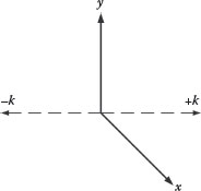
FIGURE 17.3
Momenta coordinates applicable to the PW entanglement experimental configuration.

Following a remarkable discussion that includes antisymmetrical single states, in both polarizations, and the importance of the condition of zero angular momentum, he arrives at (Ward, 1949)

$\left(|x_1,y_2\rangle -|y_1,x_2\rangle \right)\left(|+k,-k\rangle -|-k,+k\rangle \right)$

(17.46)

Ward then provides an extensive argument that selects the equation above as the likely alternative for the correct physics (Duarte, 2012). Focusing on the polarization component exclusively, we have

$\left(|x_1,y_2\rangle -|y_1,x_2\rangle \right)$

(17.47)

Using the identities given by Dirac (1978) (|x〉|y〉 = |x, y〉), this can be written as

$\left(\left|x{\rangle }_1\right|y{\rangle }_2-\left|y{\rangle }_1\right|x{\rangle }_2\right)$

(17.48)

and following normalization, we get

$\frac{1}{\sqrt{2}}{(|x\rangle }_1|y{\rangle }_2-|y{\rangle }_1|x{\rangle }_2)$

(17.49)

and its linear combination is

$\frac{1}{\sqrt{2}}{(|x\rangle }_1|y{\rangle }_2+|y{\rangle }_1|x{\rangle }_2)$

(17.50)

for quanta propagating in the opposite directions as depicted in Figure 17.4. These are the widely used equations to describe the probability amplitude of entangled polarizations of quanta propagating in opposite directions (Bohm and Aharonov, 1957; Duncan and Kleinpoppen, 1988). Since probability amplitude equations of this form were also derived independently by Snyder et al. (1948), it has been proposed that they should be named Pryce–Ward–Snyder (PWS) probability amplitudes (Duarte, 2012).

FIGURE 17.4
PW experiment for two-photon entangled polarizations. Photon 1 and photon 2 are emitted in opposite directions along the z axis, from a single source. The photons undergo Compton scattering at S₁ and S₂ thus being scattered at angles θ₁ and θ₂. The essence of this experiment consists in the following: (1) the emission of entangled photons in opposite directions, (2) the propagation of these photons in opposite directions, (3) angular selectivity at each of the propagation paths, and (4) irreversible detection at the end of each propagation path. In this regard, this experimental configuration is equivalent to that described in Figure 17.2.

In his thesis, Ward (1949) uses these probability amplitudes as an initial step in the calculation that eventually yielded the quantum ratio for perpendicular polarization over parallel polarization counting rate (Pryce and Ward, 1947).

17.5  Pryce–Ward–Snyder Probability

In order to evaluate numerically the corresponding measurable, which is the corresponding probability, we use the PWS probability amplitude

$|s\rangle =\frac{1}{\sqrt{2}}{(|x\rangle }_1|y{\rangle }_2-\left|y{\rangle }_1\right|x{\rangle }_2)$

(17.51)

in conjunction with the geometrical identities involved in rotating some generic polarization axis from x to x′ and so on (see Chapter 16):

$\langle x^{\prime }|x\rangle =\text{cos}\text{θ}$

(17.52)

$\langle y^{\prime }|x\rangle =\text{sin}\text{θ}$

(17.53)

$\langle x^{\prime }|y\rangle =-\text{sin}\text{θ}$

(17.54)

$\langle y^{\prime }|y\rangle =\text{cos}\text{θ}$

(17.55)

Thus, using Equation 17.51, the probability amplitude 〈x′|s〉 becomes

$\langle x^{\prime }|s\rangle =\frac{1}{\sqrt{2}}\left({\langle x^{\prime }|x\rangle }_1{\langle x^{\prime }|y\rangle }_2-{\langle x^{\prime }|y\rangle }_1{\langle x^{\prime }|x\rangle }_2\right)$

(17.56)

and the corresponding probability is

$|\langle x^{\prime }|s\rangle {|}^2=\frac{1}{2}{\left({\langle x^{\prime }|x\rangle }_1{\langle x^{\prime }|y\rangle }_2-{\langle x^{\prime }|y\rangle }_1{\langle x^{\prime }|x\rangle }_2\right)}^2$

(17.57)

Substituting the corresponding trigonometric terms into Equation 17.57, we get

$\begin{array}{c}|\langle x^{\prime }|s\rangle {|}^2=\frac{1}{2}{(\text{sin}{\text{θ}}_1\text{cos}{\text{θ}}_2-\text{cos}{\text{θ}}_1\text{sin}{\text{θ}}_2)}^2\\ |\langle x^{\prime }|s\rangle {|}^2=\frac{1}{2}{\text{sin}}^2({\text{θ}}_1-{\text{θ}}_2)\end{array}$

(17.58)

which allow us to evaluate numerically the probability depending on the settings θ₁ and θ₂. The PWS probability is applied to evaluate Bell’s inequality in Chapter 21.

17.6  Pryce–Ward Experimental Arrangement

The first experimental configuration including a central source emitting two correlated quanta in opposite directions is due to Pryce and Ward (1947) and is depicted in Figure 17.4. The two counterpropagating quanta undergo Compton scattering at S₁ and S₂ that causes the respective photons to be scattered at angles θ₁ and θ₂. The essence of this experiment consists in (1) the emission of entangled photons in opposite directions, (2) the propagation of these photons in opposite directions, (3) angular selectivity at each propagation path, and (4) irreversible detection at the end of each propagation path.

Duarte (2012) goes into a detailed discussion on the origin of the ideas that culminated in the PW configuration. In this regard, the first written, nondiagrammatic, description of this type of experiment was provided by Wheeler (1946), while Pryce and Ward (1947) also mention a proposal by R. C. Hanna. However, all participants appear to refer to Dirac himself as the source of the seminal idea (Duarte, 2012). Certainly, Snyder et al. (1948) also disclosed an experimental diagram that they based on Wheeler’s suggestion.

17.7  Wu–Shaknov Experiment

Following the publications of Pryce and Ward (1947) and Snyder et al. (1948), Wu and Shaknov (1950) reported experimental results on the maximum polarization ratio of the two counterpropagating quanta (2.04 ± 0.08) that was only ∼2% higher than the theoretical value, as per the PW theory. Other experimental efforts were those of Hanna (1948) and Bleuler and Bradt (1948). The literature as presented here led Dalitz and Duarte (2000) to state explicitly that the correct quantum theory for entangled quantum traveling in opposite directions was already known in 1947 and already confirmed by experiment by 1950.

17.7.1  Relevance of the Pryce–Ward Theory and the Wu–Shaknov Experiment to EPR

Here, we quote directly from relevant publications on the importance of the PWS theory and the Wu and Shaknov (WS) experiment to the Einstein, Podolsky, and Rosen (1935) (EPR) paradox (see Chapter 21).

First, in their original paper, Wu and Shaknov (1950) refer to the theory behind their experiment: “As early as 1946 J. A. Wheeler proposed an experiment to verify a prediction of pair theory, that the two quanta emitted in the annihilation of a positron–electron pair, with zero angular momentum, are polarized at right angles to each other… The detailed theoretical investigations were reported by Pryce and Ward and Snyder et al.” This is a clear and explicit statement providing a firm nexus between the PWS theory and the WS experiment.

Next is the link between the WS experiment and the EPR paradox. In this regard, Bohn and Aharanov (1957) write in reference to the WS experiment: “Thus, the paradox of EPR can equally well be tested by polarization properties of pair of photons.” Via simple deduction, if the experiment of Wu and Shaknov is considered as an EPR-type experiment, equally relevant should be the theory and experimental scheme disclosed by Pryce and Ward (Duarte, 2012).

The Bohm and Aharanov (1957) opinion on the WS experiment was questioned by some authors (Peres and Singer, 1960). However, this criticism was explicitly rejected by these authors: “In a previous paper (Bohm and Aharanov, 1957) we have discussed the paradox of Einstein, Podolsky, and Rosen (1935), and we have shown that the Wu-Shaknov experiment (Wu and Shaknov, 1950)… provides an experimental confirmation of the features of quantum mechanisms which are the basis of the above paradox” (Bohm and Aharanov, 1960).

Following the publication of the famous Bell (1964) paper, other authors argued that the WS experiment did not produce “evidence against local hidden-variable theories” given the “use of Compton polarimeters” (Clauser et al., 1969). Wu and colleagues responded that “even though a Compton experiment cannot rule out hidden-variable theories, it can provide strong evidence against them” (Kasday et al., 1975). Dalitz and Duarte (2000) also argue that the PWS theory and the WS experiment provide evidence against local realism.

From a historical perspective, it should be mentioned that the 1957 Bohm and Aharanov paper became the inspiration of researchers interested in optical experiments on entangled polarizations (see, e.g., Aspect et al. 1982).

17.8  Conclusion

The theory of entangled quantum polarizations, central to EPR-type optical experiments, was established in the 1947–1949 period by Pryce and Ward (Pryce and Ward 1947; Ward 1949) and independently by Snyder et al. (1948). Thus, it would be proper to name the expression

$|s\rangle =\frac{1}{\sqrt{2}}{(|x\rangle }_1|y{\rangle }_2-\left|y{\rangle }_1\right|x{\rangle }_2)$

as the PW probability amplitude or the PWS probability amplitude. Here, we have established that in addition to Ward’s original derivation, it is possible to arrive at this equation using the Hamiltonian approach and a direct interferometric approach.

On a broader perspective, the evidence presented here tends to indicate that the physics of quantum entanglement, as initiated by Dirac, discussed by Wheeler, and resolved by Pryce and Ward, would still be here even in the apparent absence of interpretational questions (see Chapter 21). In other words, the physics of polarization entanglement was established as a purely quantum physics result independent of interpretational efforts.

This is an observation of fundamental importance that is not widely appreciated.

Problems

17.1  Verify that substituting Equations 17.18 and 17.19 into 17.17 yields Equation 17.20.

17.2  Show that Equation 17.35 in its normalized version becomes

$|s\rangle =\frac{1}{\sqrt{2}}\left(\left|x{\rangle }_1\right|y{\rangle }_2-\left|y{\rangle }_1\right|x{\rangle }_2\right)$

17.3  Show that substitution of Equations 17.52 and 17.54 into Equation 17.56 leads to the PWS probability given in Equation 17.58

17.4  Using Equation 17.51, in conjunction with Equations 17.53 and 17.55, find the probability amplitude 〈y′|s〉.

17.5  For θ₁ = π/3 and θ₂ = π/6, evaluate the PWS probability using Equation 17.58.

References

Aspect, A., Dalibard, J., and Roger, G. (1982). Experimental test of Bell’s inequalities using time-varying analyzers. Phys. Rev. Lett. 49, 1804–1807.

Bell, J. S. (1964). On the Einstein-Podolsky-Rosen paradox. Physics 1, 195–200.

Bleuler, E. and Bradt, H. L. (1948). Correlation between the states of polarization of the two quanta of annihilation radiation. Phys. Rev. 73, 1398.

Bohm, D. and Aharonov, Y. (1957). Discussion of experimental proof for the paradox of Einstein, Rosen, and Podolsky. Phys. Rev. 108, 1070–1076.

Bohm, D. and Aharonov, Y. (1960). Further discussion of possible experimental tests for the paradox of Einstein, Podolsky and Rosen. Nouvo Cimento 17, 964–976.

Clauser, J. F., Horne, M. A., Shimony, A., and Holt, R. A. (1969). Proposed experiment to test hidden variable theories. Phys. Rev. Lett. 23, 880–884.

Dalitz, R. H. and Duarte, F. J. (2000). John Clive Ward. Phys. Today 53(10), 99–100.

Dirac, P. A. M. (1930). On the annihilation of electron and protons. Camb. Phil. Soc. 26, 361–375.

Dirac, P. A. M. (1978). The Principles of Quantum Mechanics, 4th edn. Oxford, London, U.K.

Duarte, F. J. (2012). The origin of quantum entanglement experiments based on polarization measurements. Eur. Phys. J. H 37, 311–318.

Duncan, A. J. and Kleinpoppen, H. (1988). The experimental investigation of the Einstein-Podolsky-Rosen question and Bell’s inequality. In Quantum Mechanics Versus Local Realism (Selleri, F., ed.), Plenum, New York. Chapter 7.

Einstein, A., Podolsky, B., and Rosen, N. (1935). Can quantum mechanical description of physical reality be considered complete? Phys. Rev. 47, 777–780.

Feynman, R. P., Leighton, R. B., and Sands, M. (1965). The Feynman Lectures on Physics, Vol. III, Addison-Wesley, Reading, MA.

Hanna, R. C. (1948). Polarization of annihilation radiation. Nature 162, 332.

Kasday, L. R., Hullman, J. D., and Wu, C. S. (1975). Angular correlation of Comptonscattered annihilation photons and hidden variables. Nouvo Cimento B 17, 633–661.

Mandel, L. and Wolf, E. (1995). Optical Coherence and Quantum Optics. Cambridge University, Cambridge, U.K.

Peres, A. and Singer, P. (1960). On possible experimental tests for the paradox of Einstein, Podolsky and Rosen. Nuovo Cimento 15, 907–915.

Pryce, M. H. L. and Ward, J. C. (1947). Angular correlation effects with annihilation radiation. Nature 160, 435.

Snyder, H. S., Pasternack, S., and Hornbostel, J. (1948). Angular correlation of scattered annihilation radiation. Phys. Rev. 73, 440–448.

Ward, J. C. (1949). Some Properties of the Elementary Particles. D. Phil Thesis, Oxford University, Oxford, U.K.

Wheeler, J. A. (1946). Polyelectrons. Ann. NY Acad. Sci. 48, 219–238.

Wu, C. S. and Shaknov, I. (1950). The angular correlation of scattered annihilation radiation. Phys. Rev. 77, 136.