4

Dirac Quantum Optics

4.1    Dirac Notation in Optics

The Dirac notation is one of the mathematical avenues that can be used to describe nature quantum mechanically. This mathematical notation was invented by Dirac in 1939 and is particularly well suited to describe quantum optics. In this chapter, we introduce the reader to the basics of the Dirac notation and apply the notation to the generalized description of the fundamental phenomenon of interference that, as it will be seen, is crucial to quantum physics itself. This description is based on topics and elements of a review given by Duarte (2003).

In Principles of Quantum Mechanics, first published in 1930, Dirac discusses the essence of interference as a one-photon phenomenon. Albeit his discussion is qualitative, it is also profound. In 1965, Feynman discussed electron interference via a two-slit thought experiment using probability amplitudes and the Dirac notation as a tool (Feynman et al., 1965). In 1989, inspired on Feynman’s discussion, the Dirac notation was applied to the propagation of coherent light in an N-slit interferometer (Duarte and Paine, 1989; Duarte, 1991, 1993).

The ideas of the notation invented by Dirac (1939) can be explained by considering the propagation of a photon from plane s to plane x, as illustrated in Figure 4.1. According to the Dirac concept, there is a probability amplitude, denoted by 〈x|s〉, that quantifies such propagation. Historically, Dirac introduced the nomenclature of ket vectors, denoted by | 〉, and bra vectors, denoted by 〈 |, which are mirror images of each other. Thus, the probability amplitude is described by the bra–ket 〈x|s〉, which is a complex number.

In the Dirac notation, the propagation from s to x is expressed in reverse order by 〈x|s〉. In other words, the starting position is at the right and the final position is at the left. If the propagation of the photon is not directly from plane s to plane x but involves the passage through an intermediate plane j, as illustrated in Figure 4.2, then the probability amplitude describing such propagation becomes

$\langle x|s\rangle =\langle x|j\rangle \langle j|s\rangle$

(4.1)

FIGURE 4.1
Propagation from s to the interferometric plane x is expressed as the probability amplitude 〈x|s〉. D_〈x|s〉 is the physical distance between the two planes.

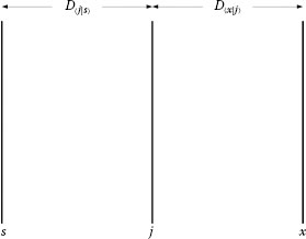
FIGURE 4.2
Propagation from s to the interferometric plane x via an intermediate plane j is expressed as the probability amplitude 〈x|s〉 = 〈x|j〉〈j|s〉. D_〈j|s〉 and D_〈x|j〉 are the distances between the designated planes.

If the photon from s must also propagate through planes j and k in its trajectory to x, that is, s→j→k→x, as illustrated in Figure 4.3, then the probability amplitude is given by

$\langle x|s\rangle =\langle x|k\rangle \langle k|j\rangle \langle j|s\rangle$

(4.2)

If an additional intermediate plane l is added, so that the propagation, from plane to plane, proceeds as s→j→k→l→x, then the probability amplitude is given by

$\langle x|s\rangle =\langle x|l\rangle \langle l|k\rangle \langle k|j\rangle \langle j|s\rangle$

(4.3)

FIGURE 4.3
Propagation from s to the interferometric plane x via two intermediate planes j and k is expressed as the probability amplitude 〈x|s〉 = 〈x|k〉〈k|j〉〈j|s〉. D_〈j|s〉, D_〈k|j〉, and D_〈x|k〉, are the distances between the designated planes.

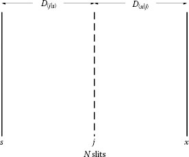
FIGURE 4.4
Propagation from s to the interferometric plane x via an array of N slits positioned at the intermediate plane j. D_〈x|j〉 is the distance between the N-slit array and the x plane.

When at the intermediate plane, in Figure 4.2, a number of N alternatives are available to the passage of the photon, as depicted in Figure 4.4, then the overall probability amplitude must consider every possible alternative, which is expressed mathematically by a summation over j in the form of

$\langle x|s\rangle ={\displaystyle \sum _{j=1}^N\langle x|j\rangle \langle j|s\rangle }$

(4.4)

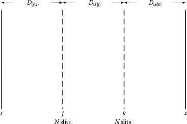
FIGURE 4.5
Propagation from s to the interferometric plane x via an array of N slits positioned at the intermediate plane j and via an additional array of N slits positioned at k. D_〈k|j〉 is the distance between the N-slit arrays.

Consideration of every possible alternative N in the computation of probability amplitude, as described in Equation 4.4, is an essential and crucial quantum feature.

For the case of an additional intermediate plane with N alternatives, as illustrated in Figure 4.5, the probability amplitude is written as

$\langle x|s\rangle ={\displaystyle \sum _{k=1}^N{\displaystyle \sum _{j=1}^N\langle x|k\rangle \langle k|j\rangle \langle j|s\rangle }}$

(4.5)

And for the case including three intermediate N-slit arrays, the probability amplitude becomes

$\langle x|s\rangle ={\displaystyle \sum _{l=1}^N{\displaystyle \sum _{k=1}^N{\displaystyle \sum _{j=1}^N\langle x|l\rangle \langle l|k\rangle \langle k|j\rangle \langle j|s\rangle }}}$

(4.6)

The addition of further intermediate planes, with N alternatives, can then be systematically incorporated in the notation. The Dirac notation albeit originally applied to the propagation of single particles (Feynman et al., 1965; Dirac, 1978) also applies to describe the propagation of ensembles of coherent, or indistinguishable, photons (Duarte, 1991, 1993, 2004). This observation is compatible with the postulate that indicates that the principles of quantum mechanics are applicable to the description of macroscopic phenomena that are not perturbed by observation (van Kampen, 1988).

4.2    Dirac Quantum Principles

The principles established by Dirac in 1939, associated to his description of quantum mechanics, via the Dirac notation, can be described rather succinctly (Feynman et al., 1965). The first principle stipulates that any state, such as ψ, can be described in terms of a set of base states. The amplitude to transition from any state to another state can be written as a sum of products, such as

$\langle x|s\rangle ={\displaystyle \sum _{i=1}^N\langle x|i\rangle \langle i|s\rangle }$

(4.7)

The base states are orthogonal. This means that the amplitude to be in one if you are in the other is zero, or

$\langle i|j\rangle ={\text{δ}}_{ij}$

(4.8)

Furthermore, the amplitude to get from one state to another directly is the complex conjugate of the reverse

${\langle x|s\rangle }^{*}=\langle s|x\rangle$

(4.9)

As a matter of formality, it should be mentioned that the space of bra–ket vectors, when the vectors are restricted to a finite length and finite scalar products, is called a Hilbert space (Dirac, 1978). However, Dirac himself points out that bra–ket vectors form a more general space than a Hilbert space (Note: a Hilbert space is a generalized Euclidean space).

4.3    Interference and the Interferometric Equation

The Dirac notation offers a natural avenue to describe the propagation of particles from a source to a detection plane, via a pair of slits. This was done by Feynman in a thought experiment using electrons and two slits. The Feynman approach was extended to the description of indistinguishable photon propagation from a source s to an interferometric plane x, via a transmission grating j comprised by N slits, as illustrated in Figure 4.6, by Duarte (1989, 1991).

In the interferometric architecture of Figure 4.6, an expanded laser beam, from a single-transverse-mode narrow-linewidth laser, becomes the radiation source (s) and illuminates an array of N slits or transmission grating (j). The interaction of the coherent radiation with the N-slit array (j) produces an interference signal at x. A crucial point here is that all the indistinguishable photons illuminate the array of N slits, or grating, simultaneously. If only one photon propagates, at any given time, then that individual photon illuminates the whole array of N slits simultaneously (Duarte, 2003). The probability amplitude that describes the propagation from the source (s) to the detection plane (x), via the array of N slits (j), is given by (Duarte, 1991, 1993)

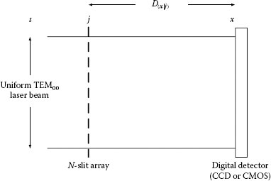
FIGURE 4.6
N-slit laser interferometer: A near-Gaussian beam from a single transverse mode (TEM₀₀), narrow-linewidth laser is preexpanded in 2D telescope and then expanded in one dimension (parallel to the plane of incidence) by an MPBE (Duarte, 1987). This expanded beam can be further transformed into a nearly uniform illumination source (s) (Duarte, 2003). Then, a uniform light source (s) illuminates an array of N slits at j. Interaction of the coherent emission with the slit array produces interference at the interferometric plane x (Duarte, 1993).

$\langle x|s\rangle ={\displaystyle \sum _{j=1}^N\langle x|j\rangle \langle j|s\rangle }$

According to Dirac (1978), the probability amplitudes can be represented by wave functions of ordinary wave optics. Thus, following Feynman et al. (1965),

$\langle j|s\rangle =\text{Ψ}(r_{j,s})e^{-i{\text{θ}}_j}$

(4.10)

$\langle x|j\rangle =\text{Ψ}(r_{x,j})e^{-i{\text{ϕ}}_j}$

(4.11)

where θ_j and ϕ_j are the phase terms associated with the incidence and diffraction waves, respectively. Using Equations 4.10 and 4.11, for the probability amplitudes, the propagation probability amplitude

$\langle x|s\rangle ={\displaystyle \sum _{j=1}^N\langle x|j\rangle \langle j|s\rangle }$

can be written as

$\langle x|s\rangle ={\displaystyle \sum _{j=1}^N\text{Ψ}(r_j)e^{-i{\text{Ω}}_j}}$

(4.12)

where

$\text{Ψ}(r_j)=\text{Ψ}(r_{x,j})\text{Ψ}(r_{j,s})$

(4.13)

and

${\text{Ω}}_j=({\text{θ}}_j+{\text{ϕ}}_j)$

(4.14)

Next, the propagation probability is obtained by expanding Equation 4.12 and multiplying the expansion by its complex conjugate, or

$|\langle x|s\rangle {|}^2=\langle x|s\rangle {\langle x|s\rangle }^{*}$

(4.15)

Expansion of the probability amplitude and multiplication with its complex conjugate, following some algebra, lead to

$|\langle x|s\rangle {|}^2={\displaystyle \sum _{j=1}^N\text{Ψ}(r_j)}{\displaystyle \sum _{m=1}^N\text{Ψ}(r_m)e^{i({\text{Ω}}_m-{\text{Ω}}_j)}}$

(4.16)

Expanding Equation 4.16 and using the identity

$2\text{ cos }({\text{Ω}}_m-{\text{Ω}}_j)=e^{-i({\text{Ω}}_m-{\text{Ω}}_j)}+e^{i({\text{Ω}}_m-{\text{Ω}}_j)}$

(4.17)

lead to the explicit form of the generalized propagation probability in one dimension (Duarte and Paine, 1989; Duarte, 1991):

$|\langle x|s\rangle {|}^2={\displaystyle \sum _{j=1}^N\text{Ψ}{(r_j)}^2}+2{\displaystyle \sum _{j=1}^N\text{Ψ}(r_j)\left({\displaystyle \sum _{m=j+1}^N\text{Ψ}(r_m)\text{ cos }({\text{Ω}}_m-{\text{Ω}}_j)}\right)}$

(4.18)

This equation is the 1D generalized interferometric equation. The reader should keep in mind that it is completely equivalent to Equation 4.16.

4.3.1    Examples: Double-, Triple-, Quadruple-, and Quintuple-Slit Interference

Expanding Equation 4.16 for two slits (N = 2), as applicable to double-slit interference, we get

$\begin{array}{ll}|\langle x|s\rangle {|}^2\hfill & =\text{Ψ}(r_1)(\text{Ψ}(r_1)e^{i({\text{Ω}}_1-{\text{Ω}}_1)}+\text{Ψ}(r_2)e^{i({\text{Ω}}_2-{\text{Ω}}_1)})+\text{Ψ}(r_2)(\text{Ψ}(r_1)e^{i({\text{Ω}}_1-{\text{Ω}}_2)}+\text{Ψ}(r_2)e^{i({\text{Ω}}_2-{\text{Ω}}_2)})\hfill \\ |\langle x|s\rangle {|}^2\hfill & =\text{Ψ}(r_1)(\text{Ψ}(r_1)+\text{Ψ}(r_2)e^{i({\text{Ω}}_2-{\text{Ω}}_1)})+\text{Ψ}(r_2)(\text{Ψ}(r_1)e^{i({\text{Ω}}_1-{\text{Ω}}_2)}+\text{Ψ}(r_2))\hfill \\ |\langle x|s\rangle {|}^2\hfill & =\text{Ψ}{(r_1)}^2+\text{Ψ}{(r_2)}^2+(\text{Ψ}(r_1)\text{Ψ}(r_2)e^{i({\text{Ω}}_2-{\text{Ω}}_1)}+\text{Ψ}(r_1)\text{Ψ}(r_2)e^{i({\text{Ω}}_1-{\text{Ω}}_2)})\hfill \\ |\langle x|s\rangle {|}^2\hfill & =\text{Ψ}{(r_1)}^2+\text{Ψ}{(r_2)}^2+(\text{Ψ}(r_1)\text{Ψ}(r_2)e^{i({\text{Ω}}_2-{\text{Ω}}_1)}+\text{Ψ}(r_1)\text{Ψ}(r_2)e^{-i({\text{Ω}}_2-{\text{Ω}}_1)})\hfill \\ |\langle x|s\rangle {|}^2\hfill & =\text{Ψ}{(r_1)}^2+\text{Ψ}{(r_2)}^2+2\text{Ψ}(r_1)\text{Ψ}(r_2)\text{ cos }({\text{Ω}}_2-{\text{Ω}}_1)\hfill \end{array}$

(4.19)

Expanding Equation 4.18 for three slits (N = 3), applicable to triple-slit interference, we get

$|\langle x|s\rangle {|}^2=\text{Ψ}{(r_1)}^2+\text{Ψ}{(r_2)}^2+\text{Ψ}{(r_3)}^2+2(\text{Ψ}(r_1)\text{Ψ}(r_2)\text{ cos }({\text{Ω}}_2-{\text{Ω}}_1)+\text{Ψ}(r_1)\text{Ψ}(r_3)\text{ cos }({\text{Ω}}_3-{\text{Ω}}_1)+\text{Ψ}(r_2)\text{Ψ}(r_3)\text{ cos }({\text{Ω}}_3-{\text{Ω}}_2))$

(4.20)

Expanding Equation 4.18 for four slits (N = 4), applicable to quadruple-slit interference, we get

$|\langle x|s\rangle {|}^2=\text{Ψ}{(r_1)}^2+\text{Ψ}{(r_2)}^2+\text{Ψ}{(r_3)}^2+\text{Ψ}{(r_4)}^2+2(\text{Ψ}(r_1)\text{Ψ}(r_2)\text{ cos }({\text{Ω}}_2-{\text{Ω}}_1)+\text{Ψ}(r_1)\text{Ψ}(r_3)\text{ cos }({\text{Ω}}_3-{\text{Ω}}_1)+\text{Ψ}(r_1)\text{Ψ}(r_4)\text{ cos }({\text{Ω}}_4-{\text{Ω}}_1)+\text{Ψ}(r_2)\text{Ψ}(r_3)\text{ cos }({\text{Ω}}_3-{\text{Ω}}_2)+\text{Ψ}(r_2)\text{Ψ}(r_4)\text{ cos }({\text{Ω}}_4-{\text{Ω}}_2)+\text{Ψ}(r_3)\text{Ψ}(r_4)\text{ cos }({\text{Ω}}_4-{\text{Ω}}_3))$

(4.21)

Expanding Equation 4.18 for five slits (N = 5), applicable to quintuple-slit interference, we get

$|\langle x|s\rangle {|}^2=\text{Ψ}{(r_1)}^2+\text{Ψ}{(r_2)}^2+\text{Ψ}{(r_3)}^2+\text{Ψ}{(r_4)}^2+\text{Ψ}{(r_5)}^2+2(\text{Ψ}(r_1)\text{Ψ}(r_2)\text{ cos }({\text{Ω}}_2-{\text{Ω}}_1)+\text{Ψ}(r_1)\text{Ψ}(r_3)\text{ cos }({\text{Ω}}_3-{\text{Ω}}_1)+\text{Ψ}(r_1)\text{Ψ}(r_4)\text{ cos }({\text{Ω}}_4-{\text{Ω}}_1)+\text{Ψ}(r_1)\text{Ψ}(r_5)\text{ cos }({\text{Ω}}_5-{\text{Ω}}_1)+\text{Ψ}(r_2)\text{Ψ}(r_3)\text{ cos }({\text{Ω}}_3-{\text{Ω}}_2)+\text{Ψ}(r_2)\text{Ψ}(r_4)\text{ cos }({\text{Ω}}_4-{\text{Ω}}_2)+\text{Ψ}(r_2)\text{Ψ}(r_5)\text{ cos }({\text{Ω}}_5-{\text{Ω}}_2)+\text{Ψ}(r_3)\text{Ψ}(r_4)\text{ cos }({\text{Ω}}_4-{\text{Ω}}_3)+\text{Ψ}(r_3)\text{Ψ}(r_5)\text{ cos }({\text{Ω}}_5-{\text{Ω}}_3)+\text{Ψ}(r_4)\text{Ψ}(r_5)\text{ cos }({\text{Ω}}_5-{\text{Ω}}_4))$

(4.22)

and so on. Besides the explicit interferometric expressions for N = 2, N = 3, N = 4, and N = 5, Equation 4.18 can be programmed to include sextuple (N = 6), septuple (N = 7), octuple (N = 8), nonuple (N = 9), or any number of slits, and in practice it has been used to do calculations, and comparisons with measurements, in the 2 ≤ N ≤ 2000 range (Duarte, 1993, 2009).

4.3.2    Geometry of the N-Slit Interferometer

The relevant geometry, and geometrical parameters, at the transmission grating (j) and the plane of interference (x) are illustrated in Figures 4.6, Figures 4.7, 4.8. According to the geometry, the phase difference term in Equations 4.16 and 4.18 can be expressed as (Duarte, 1997)

$\text{ cos }(({\text{θ}}_m-{\text{θ}}_j)\pm ({\text{ϕ}}_m-{\text{ϕ}}_j))=\text{ cos }(|l_m-l_{m-1}|k_1\pm |L_m-L_{m-1}|k_2)$

(4.23)

where

$k_1=\frac{2\text{π}{n}_1}{{\text{λ}}_v}$

(4.24)

and

$k_2=\frac{2\text{π}{n}_2}{{\text{λ}}_v}$

(4.25)

are the wave numbers of the two optical regions defined in Figure 4.8. Here, λ₁ = λ_v/n₁ and λ₂ = λ_v/n₂ where λ_v is the vacuum wavelength, while n₁ and n₂ are the corresponding indexes of refraction (Wallenstein and Hänsch, 1974; Born and Wolf, 1999). The phase differences are expressed exactly via the following geometrical equations (Duarte, 1993):

$|L_m-L_{m-1}|=\frac{2{\text{ξ}}_m{d}_m}{|L_m+L_{m-1}|}$

(4.26)

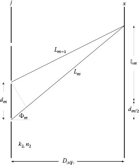
FIGURE 4.7
The N-slit array, or transmission grating, plane (j) and the interferometric plane (x) (not to scale) illustrating the path difference and the various parameters involved in the exact description of the geometry.

$L_m^2=D_{\langle x|j\rangle }^2+{\left({\text{ξ}}_m+\frac{d_m}{2}\right)}^2$

(4.27)

$L_{m-1}^2=D_{\langle x|j\rangle }^2+{\left({\text{ξ}}_m-\frac{d_m}{2}\right)}^2$

(4.28)

In this notation ξ_m is the lateral displacement, on the x plane, from the projected median of d_m to the interference plane, and D_〈x|j〉 is the intra-interferometric distance from the j plane to the x plane. Accurate representation of the exact geometry is important when writing software to generate numerical interferograms based on Equation 4.18.

4.3.3    Diffraction Grating Equation

In the phase term equation

$\text{ cos }(({\text{θ}}_m-{\text{θ}}_j)\pm ({\text{ϕ}}_m-{\text{ϕ}}_j))=\text{ cos }(|l_m-l_{m-1}|k_1\pm |L_m-L_{m-1}|k_2)$

the corresponding path differences are |l_m − l_m−1| and |L_m − L_m−1|. Since maxima occur at

$(|l_m-l_{m-1}|n_1\pm |L_m-L_{m-1}|n_2)\frac{2\text{π}}{{\text{λ}}_v}=M\text{π}$

(4.29)

FIGURE 4.8
Close up of the N-slit array, or transmission grating, plane (j) illustrating the path length difference and the angles of incidence (Θ_m) and diffraction (Φ_m) for the condition D_〈x|j〉 ≫ d_m as described. (Reproduced from Duarte, F.J., Am. J. Phys. 65, 637, 1997, with permission from the American Association of Physics Teachers.)

where M = 0, ±2, ±4, ±6 ⋯, it can be shown that

$d_m(n_1\text{ sin }{\text{Θ}}_m\pm n_2\text{ sin }{\text{Φ}}_m)\frac{2\text{π}}{{\text{λ}}_v}=M\text{π}$

(4.30)

which, for n₁ = n₂ = 1 and λ = λ_v, reduces to

$d_m(\text{sin }{\text{Θ}}_m\pm \text{sin }{\text{Φ}}_m)k=M\text{π}$

(4.31)

that can be expressed as the well-known grating equation

$d_m(\text{sin }{\text{Θ}}_m\pm \text{sin }{\text{Φ}}_m)=m\text{λ}$

(4.32)

where m = 0, ±1, ±2, ±3 ⋯. For a grating utilized in the reflection domain, in Littrow configuration, Θ_m = Φ_m = Θ so that the grating equation reduces to

$2d\text{sin }\text{Θ}=m\text{λ}$

(4.33)

These diffraction equations are reconsidered, in a more general form, with an extra sign alternative in Chapter 5.

4.3.4    N-Slit Interferometer Experiment

The N-slit interferometer is illustrated in Figure 4.9. In practice this interferometer can be configured with a variety of lasers including tunable lasers. However, one requirement is that the laser to be utilized must emit in the narrow-linewidth regime and in a single transverse mode (TEM₀₀) with a near-Gaussian profile. Ideally the source should be a single-longitudinalmode laser (see Chapter 9). The reason for this requirement is that narrowlinewidth lasers yield sharp well-defined interference patterns close to those predicted theoretically for a single wavelength.

One particular configuration of the N-slit laser interferometer (NSLI), described by Duarte (1993), utilizes a TEM₀₀ He–Ne laser (λ ≈ 632.82 nm) with a beam 0.5 mm in diameter as the illumination source. This class of laser yields a smooth near-Gaussian beam profile and narrow-linewidth emission (∆ν ≈ 1 GHz). The laser beam is then magnified, in two dimensions, by a Galilean telescope. Following the telescopic expansion, the beam is further expanded, in one dimension, by a multiple-prism beam expander (MPBE). This class of optical architecture can yield an expanded smooth near-Gaussian beam approximately 50 mm wide. An option is to insert a convex lens prior to the multiple-prism expander thus producing an extremely elongated near-Gaussian beam (Duarte, 1987, 1993). The beam propagation through this system can be accurately characterized using ray transfer matrices as discussed in Duarte (2003) (see Appendix C). Also, as an option, at the exit of the MPBE, an aperture, a few mm wide, can be deployed.

The beam profile thus produced can be neatly reproduced by the interferometric equation as illustrated later in this chapter. Thus, the source s can be either the exit prism of the MPBE or the wide aperture. For the results discussed in this chapter, on the detection side, the interference screen at x is a digital detector comprised of a photodiode array with individual pixels each 25 μm in width.

FIGURE 4.9
Top view schematics of the N-slit interferometer. A neutral density filter follows the TEM₀₀ narrow linewidth. The laser beam is then magnified in two dimensions by a telescope beam expander (TBE). The magnified beam is then expanded in one dimension by an MPBE. A wide aperture then selects the central part of the expanded beam to illuminate the N-slit array (j). The interferogram then propagates via the intra-interferometric path D_〈x|j〉 in its ways toward the interference plane x. Detection of the interferogram at x can either be performed by a silver halide film or a digital array such as a CCD or CMOS detector. (Reproduced from Duarte, F.J. et al., J. Opt. 12, 015705, 2010, with permission from the Institute of Physics.)

Now, we consider a series of cases that demonstrate the measurement capability of the NSLI and the ability of the generalized interferometric equation to either predict or reproduce the measurement. The first case considered is the well-known double-slit experiment also known as Young’s interference experiment. For (N = 2) with slits 50 μm in width, separated by 50 μm, the elongated Gaussian beam provides a nearly plane illumination. That is also approximately the case even if a larger number of slits, of these dimensions, are illuminated. For the particular case of a two-slit experiment involving 50 μm slits separated by 50 μm and a grating to screen distance D_〈x|j〉 = 10 cm, the interference signal is displayed in Figure 4.10a. The calculated interference, using Equation 4.18, and assuming plane wave illumination are given in Figure 4.10b.

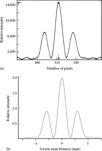
FIGURE 4.10
(a) Measured interferogram resulting from the interaction of coherent laser emission at λ = 632.82 nm and two slits (N = 2) 50 μm wide, separated by 50 μm. The j to x distance is D_〈x|j〉 = 10 cm. Each pixel is 25 μm wide. (b) Corresponding theoretical interferogram from Equation 4.18.

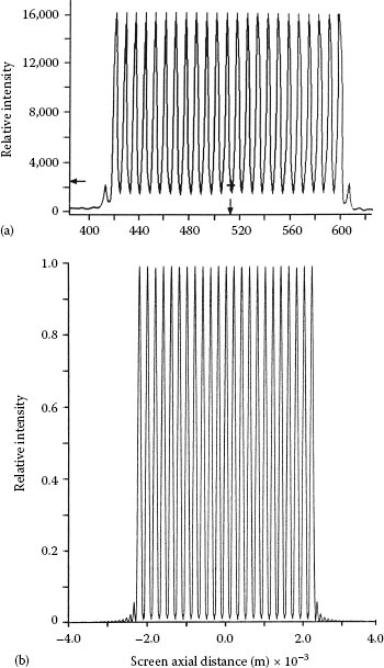
FIGURE 4.11
(a) Measured interferogram, in the near field, resulting from the interaction of coherent laser emission at λ = 632.82 nm and N = 23 slits, 100 μm wide, separated by 100 μm. Here, D_〈x|j〉 = 1.5 cm. (b) Corresponding near-field theoretical interferogram from Equation 4.18. (Reproduced from Duarte, F.J., Opt. Commun. 103, 8, 1993, with permission from Elsevier.)

For an array of N = 23 slits, each 100 μm in width and separated by 100 μm, the measured and calculated interferograms are shown in Figure 4.11. Here the grating to digital detector distance is D_〈x|j〉 = 1.5 cm. This is a near field result and corresponds entirely to the interferometric regime.

For an array of N = 100 slits, each 30 μm in width and separated by 30 μm, the measured and calculated interferograms are shown in Figure 4.12. Here the grating to digital detector distance is D_〈x|j〉 = 75 cm. In Figure 4.12 the ±1 diffraction orders are present.

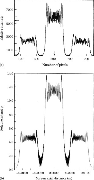
FIGURE 4.12
(a) Measured interferogram resulting from the interaction of coherent laser emission at λ = 632.82 nm and N = 100, slits 30 μm wide, separated by 30 μm. Here, D_〈x|j〉 = 75 cm. (b) Corresponding theoretical interferogram from Equation 4.18. (Reproduced from Duarte, F.J., Opt. Commun. 103, 8, 1993, with permission from Elsevier.)

In practice, the transmission gratings are not perfect and offer an uncertainty in the dimension of the slits. The uncertainty in the slit dimensions of the grating, incorporating the 30 μm slits, used in this experiments was measured to be ≤2%. The theoretical interferogram for the grating comprised by N = 100 slits, each 30.0 ± 0.6 μm wide and separated by 30.0 ± 0.6 μm, is given in Figure 4.13. Notice the symmetry deterioration.

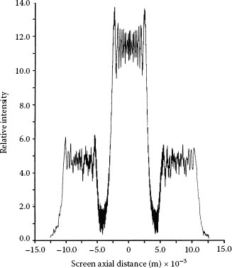
FIGURE 4.13
Theoretical interferometric/diffraction distribution using a ≤2% uncertainty in the dimensions of the 30 μm slits. In this calculation, N = 100 and D_〈x|j〉 = 75 cm. A deterioration in the spatial symmetry of the distribution is evident. (Reproduced from Duarte, F.J., Opt. Commun. 103, 8, 1993, with permission from Elsevier.)

When a wide slit is used to select the central portion of the elongated Gaussian beam, the interaction of the coherent laser beam with the slit results in diffraction prior to the illumination of the transmission grating. The interferometric Equation 4.18 can be used to characterize this diffraction. This is done by dividing the wide slit in hundreds of smaller slits. As an example a 4 mm wide aperture is divided into 800 slits each 4 μm wide and separated by a 1 μm interslit distance (Duarte, 1993). The calculated near-field diffraction pattern, for a distance of D_〈x|j〉 = 10 cm, is shown in Figure 4.14. Using this as the radiation source to illuminate the N = 100 slit grating, comprised of 30 μm slits with an interslit distance of 30 μm (for D_〈x|j〉 = 75 cm), yields the theoretical interferogram displayed in Figure 4.15. This is a cascade interferometric technique in which the interferometric distribution in one plane is used to illuminate an N-slit array in the immediately following plane and is applied further in the results discussed in Chapter 20.

FIGURE 4.14
Theoretical near-field diffraction distribution produced by a 4 mm aperture illuminated at λ = 632.82 nm, and D_〈x|j〉 = 10 cm. (Reproduced from Duarte, F.J., Opt. Commun. 103, 8, 1993, with permission from Elsevier.)

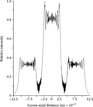
FIGURE 4.15
Theoretical interferometric distribution incorporating diffraction-edge effects in the illumination. In this calculation, the width of the slits in the array is 30 μm, separated by 30 μm, N = 100, and D_〈x|j〉 = 75 cm. The aperture-grating distance is 10 cm. (Reproduced from Duarte, F.J., Opt. Commun. 103, 8, 1993, with permission from Elsevier.)

4.4    Coherent and Semicoherent Interferograms

The interferometric equation

$|\langle x|s\rangle {|}_{\text{λ}}^2={\displaystyle \sum _{j=1}^N\text{Ψ}{(r_j)}_{\text{λ}}^2}+2{\displaystyle \sum _{j=1}^N\text{Ψ}{(r_j)}_{\text{λ}}}\left({\displaystyle \sum _{m=j+1}^N\text{Ψ}{(r_m)}_{\text{λ}}\text{ cos }({\text{Ω}}_m-{\text{Ω}}_j)}\right)$

(4.34)

was originally derived to account for single-photon propagation only (Duarte, 1993, 2004). This is illustrated by adding a single-wavelength subscript to Equation 4.18, as made explicit now in Equation 4.34. Thus, this equation is intrinsically related to monochromatic and/or highly coherent emission. In practice it has also been found that it accounts for the propagation of ensembles of indistinguishable photons or narrow-linewidth emission as available from narrow-linewidth laser sources (Duarte, 1993, 2003). The question then arises on the applicability of Equation 4.34 to the case of semicoherent, partially coherent, or broadband emission.

Equation 4.34 provides an interferogram for a single wavelength and in practice for an ensemble of indistinguishable photons. These interferograms are narrow and spatially sharp and well defined. For broadband emission, or semicoherent emission, the sharpness of the interferogram diminishes and the interferometric pattern becomes broad and less defined. This is how this occurs: each wavelength has a unique interferometric signature defined by Equation 4.34. A detector registers that signature. If the emission is broadband or semicoherent, a multitude of different interferograms are generated, and the detector (either digital or a photographic plaque) provides an integrated picture of a composite interferogram produced by the array of wavelengths involved in the emission.

Thus, for broadband emission Equation 4.34 is modified to include a sum over the wavelength range involved, so that

${\displaystyle \sum _{\text{λ}={\text{λ}}_1}^{{\text{λ}}_n}|\langle x|s\rangle {|}_{\text{λ}}^2}={\displaystyle \sum }_{\text{λ}={\text{λ}}_1}^{{\text{λ}}_n}\left({\displaystyle \sum }_{j=1}^N\text{Ψ}{(r_j)}_{\text{λ}}^2+2{\displaystyle \sum }_{j=1}^N\text{Ψ}{(r_j)}_{\text{λ}}\left({\displaystyle \sum }_{m=j+1}^N\text{Ψ}{(r_m)}_{\text{λ}}\text{ cos }({\text{Ω}}_m-{\text{Ω}}_j)\right)\right)$

(4.35)

The concept just described has been previously outlined by Duarte (2007, 2008) and is further illustrated next. In Figure 4.16 the double-slit interferogram produced with narrow-linewidth emission from the 3s₂ − 2p₁₀ transition of a He–Ne laser, at λ ≈ 543.3 nm, is displayed. The visibility of this interferogram is calculated using (Michelson, 1927)

$\nu =\frac{I_1-I_2}{I_1+I_2}$

(4.36)

FIGURE 4.16
Measured double-slit interferogram generated with He–Ne laser emission from the 3s₂ − 2p₁₀ transition at λ ≈ 543.3 nm. Here, N = 2 for a slit width of 50 μm. The intra-interferometric distance is D_〈x|j〉 = 10 cm. (Reproduced from Duarte, F.J., Opt. Lett. 32, 412, 2007, with permission from the Optical Society of America.)

FIGURE 4.17
Measured double-slit interferogram generated with emission from an organic semiconductor interferometric emitter at λ ≈ 540 nm. Here, N = 2 for a slit width of 50 μm. The intra-interferometric distance is D_〈x|j〉 = 10 cm. (Reproduced from Duarte, F.J., Opt. Lett. 32, 412, 2007, with permission from the Optical Society of America.)

to be V ≈ 0.95. In Figure 4.17 the double-slit interferogram produced, under identical geometrical conditions, but with the emission from an electrically excited coherent organic semiconductor interferometric emitter, at λ ≈ 540 nm, is displayed. Here the visibility is lower V ≈ 0.90. A comparison between the two interferograms reveals that the second interferogram has slightly broader spatial features relative to the interferogram produced with illumination from the 3s₂ − 2p₁₀ transition of the He–Ne laser. The differences in spatial distributions between these two interferograms have been used to estimate the linewidth of the emission from the interferometric emitter (Duarte, 2008).

A double-slit interferogram produced, under identical geometrical conditions, but with the emission from a broadband semicoherent source, centered around λ ≈ 540 nm, yields a visibility of V ≈ 0.55. A survey of measured double-slit interferogram visibilities from relevant semicoherent, or partially coherent, sources reveals a visibility range of 0.4 ≤ V ≤ 0.65. On the other hand, the visibility range for double-slit interferograms originating from various laser sources is 0.85 ≤ V ≤ 0.99 (Duarte, 2008).

4.5    Interferometric Equation in Two and Three Dimensions

The 2D interferometric case can be described considering a diffractive grid, or 2D N-slit array, as depicted in Figure 4.18. Photon propagation takes place from s to the interferometric plane x via a 2D transmission grating j_zy, that is, j is replaced by a grid comprised of j components in the y direction and j components in the z direction. Note that in the 1D case only the y component of j is present, which is written simply as j. The plane configured by the j_zy grid is orthogonal to the plane of propagation. Hence, for photon propagation from s to x, via j_zy, the probability amplitude is given by (Duarte, 1995)

FIGURE 4.18
Two-dimensional depiction of the interferometric system 〈x|j〉〈j|s〉. (Adapted from Duarte, F.J., Interferometric imaging, In: Tunable Laser Applications, Duarte, F. J. (ed.), Marcel Dekker, New York, 1995.)

$\langle x|s\rangle ={\displaystyle \sum }_{j_z=1}^N{\displaystyle \sum }_{j_y=1}^N\langle x|j_{zy}\rangle \langle j_{zy}|s\rangle$

(4.37)

Now, if the j is abstracted from j_zy, then Equation 4.37 can be expressed as

$\langle x|s\rangle ={\displaystyle \sum }_{z=1}^N{\displaystyle \sum }_{y=1}^N\text{Ψ}(r_{zy})e^{-i{\text{Ω}}_{zy}}$

(4.38)

and the corresponding probability is given by (Duarte, 1995)

$|\langle x|s\rangle {|}^2={\displaystyle \sum }_{z=1}^N{\displaystyle \sum }_{y=1}^N\text{Ψ}(r_{zy}){\displaystyle \sum }_{q=1}^N{\displaystyle \sum }_{p=1}^N\text{Ψ}(r_{pq})e^{i({\text{Ω}}_{\eta p}-{\text{Ω}}_{zy})}$

(4.39)

For a 3D transmission grating, it can be shown that

$|\langle x|s\rangle {|}^2={\displaystyle \sum }_{z=1}^N{\displaystyle \sum }_{y=1}^N{\displaystyle \sum }_{x=1}^N\text{Ψ}(r_{zyx}){\displaystyle \sum }_{q=1}^N{\displaystyle \sum }_{p=1}^N{\displaystyle \sum }_{r=1}^N\text{Ψ}(r_{qpr})e^{i({\text{Ω}}_{qpr}-{\text{Ω}}_{zyx})}$

(4.40)

It is important to emphasize that the equations described here apply either to the propagation of single photons or to the propagation of ensembles of coherent, indistinguishable, or monochromatic photons. For broadband emission, as described in the previous section, an interferometric summation over the emission spectrum is necessary.

The application of quantum principles to the description of propagation of a large number of monochromatic, or indistinguishable, photons was already advanced by Dirac in his discussion of interference (Dirac, 1978; Duarte, 1998).

4.6    Classical and Quantum Alternatives

Increasingly the field of optics has seen a transition from a classical description to a quantum description. Some phenomena is purely quantum and cannot be described classically. Other phenomena, such as polarization and interference, can be described either classically or quantum mechanically. In the case of interference, and diffraction, the beauty is that the quantum mechanical description also applies to the description of ensembles of indistinguishable photons. Also, when we describe interference and diffraction using quantum mechanical tools, all we are doing is following the steps of giants such as Dirac (1978) and Feynman (see, Feynman and Hibbs, 1965) (Note: Dirac’s description comes from the 1930s, but the book edition we are using is 1978).

As we shall see in Chapter 5, there is another powerful reason to describe interference quantum mechanically: This description provides a unified avenue to the whole of optics in a succinct inverse hierarchy that goes

INTERFERENCE → DIFFRACTION → REFRACTION → REFLECTION

(Duarte, 1997). By contrast the situation from a traditional classical perspective is rather disjointed as can be observed by perusing any good book on classical optics. There, the description goes like reflection, refraction, diffraction, and interference in a non-cohesive manner. Classically, there is no mathematical coherence in the description.

Furthermore, in our quantum description, a single equation is used to describe interference, and interference–diffraction phenomena, in the near and the far field in a unified manner (Duarte, 1993).

Problems

4.1  Show that substitution of Equations 4.10 and 4.11 into Equation 4.4 leads to Equation 4.12.

4.2  Show that Equation 4.16 can be expressed as Equation 4.18.

4.3  From the geometry of Figure 4.7, derive Equations 4.26, Equations 4.27, 4.28.

4.4  Write an equation for |〈x|s〉|² in the case relevant to N = 3 starting from Equation 4.16.

4.5  Write an equation for |〈x|s〉|² using the probability amplitude given in Equation 4.5.

References

Born, M. and Wolf, E. (1999). Principles of Optics, 7th edn. Cambridge, New York.

Dirac, P. A. M. (1939). A new notation for quantum mechanics. Math. Proc. Cam. Phil. Soc. 35, 416–418.

Dirac, P. A. M. (1978). The Principles of Quantum Mechanics, 4th edn. Oxford, London, U.K.

Duarte, F. J. (1987). Beam shaping with telescopes and multiple-prism beam expanders. J. Opt. Soc. Am. A 4, p30.

Duarte, F. J. (1991). Dispersive dye lasers. In High Power Dye Lasers, (Duarte, F. J., ed.). Springer-Verlag, Berlin, Germany, Chapter 2.

Duarte, F. J. (1993). On a generalized interference equation and interferometric measurements. Opt. Commun. 103, 8–14.

Duarte, F. J. (1995). Interferometric imaging. In Tunable Laser Applications, (Duarte, F. J., ed.). Marcel Dekker, New York, Chapter 5.

Duarte, F. J. (1997). Interference, diffraction, and refraction, via Dirac’s notation. Am. J. Phys. 65, 637–640.

Duarte, F. J. (1998). Interference of two independent sources. Am. J. Phys. 66, 662–663.

Duarte, F. J. (2003). Tunable Laser Optics. Elsevier-Academic, New York.

Duarte, F. J. (2004). Comment on “Reflection, refraction and multislit interference”. Eur. J. Phys. 25, L57–L58.

Duarte, F. J. (2007). Coherent electrically-excited organic semiconductors: Visibility of interferograms and emission linewidth, Opt. Lett. 32, 412–414.

Duarte, F. J. (2008). Coherent electrically excited organic semiconductors: Coherent or laser emission? Appl. Phys. B 90, 101–108.

Duarte, F. J. (2009). Interferometric imaging. In Tunable Laser Applications, 2nd edn. (Duarte, F. J., ed.). CRC, New York, Chapter 12.

Duarte, F. J. and Paine, D. J. (1989). Quantum mechanical description of N-slit interference phenomena, in Proceedings of the International Conference on Lasers’88 (Sze, R. C. and Duarte, F. J., eds.). STS Press, McLean, VA, pp. 42–47.

Duarte, F. J., Taylor, T. S., Clark, A. B., and Davenport, W. E. (2010). The N-slit interferometer: An extended configuration. J. Opt. 12, 015705.

Feynman. R. P. and Hibbs, A. R. (1965). Quantum Mechanics and Path Integrals, Mc Graw-Hill, New York.

Feynman, R. P., Leighton, R. B., and Sands, M. (1965). The Feynman Lectures on Physics, Vol. III, Addison-Wesley, Reading, MA.

Michelson, A. A. (1927). Studies in Optics, University of Chicago, Chicago, IL.

van Kampen, N. G. (1988). Ten theorems about quantum mechanical measurements. Physica A 153, 97–113.

Wallenstein, R. and Hänsch, T. W. (1974). Linear pressure tuning of a multielement dye laser spectrometer. Appl. Opt. 13, 1625–1628.