12

Schrödinger’s Equation

12.1  Introduction

As mentioned in Chapter 1, Schrödinger’s equation provides one of the three main avenues to quantum mechanics. It also has important applications in atomic and molecular physics (Herzberg, 1950; Feynman et al., 1965). Given the importance of this equation, here we examine several derivational approaches. The principal aim is to gain an understanding on the physics behind this quantum wave equation. Since the application of this equation is widely and extensively treated in many textbooks (see, e.g., Saleh and Teich, 1991; Silfvast, 2008; Hooker and Webb, 2010), here we only briefly describe a few applications relevant to semiconductor lasers.

12.2  Schrödinger’s Mind

As its name suggests, Schrödinger’s equation is the brain child of Schrödinger and was first disclosed in 1926 in a paper entitled An Undulatory Theory of the Mechanics of Atoms and Molecules (Schrödinger, 1926). The word undulatory is based on the word onde that means wave. In that extraordinary paper, Schrödinger begins with a discussion of classical kinetic energy and work. Schrödinger’s paper is not all that transparent, and it includes some imaginative arguments that are crucial to the successful development of his theory.

Next, we present Schrödinger’s argument in a very abbreviated format and with some changes in notation to improve transparency.

Schrödinger begins by considering the dynamics of a particle moving through a force field. Thus he first introduces the kinetic energy as

$T=\frac{1}{2}m\left(v_x^2+v_y^2+v_z^2\right)$

(12.1)

and he also introduces the Hamiltonian of action W

$\text{W}={\displaystyle \underset{0}{\overset{t}{\int }}(T-V)dt}$

(12.2)

which satisfies the Hamiltonian partial differential equation

$\frac{\partial W}{\partial t}+\frac{1}{2m}{(\nabla W)}^2+V(x,y,z)=0$

(12.3)

To solve this differential equation, he then tries a solution of the form

$W=-Et+S(x,y,z)$

(12.4)

Differentiating Equation 12.4, he arrives at ∂W/∂t = −E, and substitution into Equation 12.3 yields

$|\nabla W|={(2m(E-V))}^{1/2}$

(12.5)

As it will be seen later, the appearance of the 2m(E − V) term is crucial to the final Schrödinger result.

Next, Schrödinger uses Equations 12.4 and 12.5 in conjunction with a geometrical argument to obtain a “phase” velocity u:

$u=E{(2m(E-V))}^{-1/2}$

(12.6)

Equation 12.6 is an essential component of the classical part of the Schrödinger’s argument. He then introduces the quantum component via Planck’s quantum energy equation (Planck, 1901)

$E=hv$

(12.7)

and de Broglie’s quantum momentum expression (de Broglie, 1923)

$p=\frac{h}{\text{λ}}$

(12.8)

which is also based on E = hν. This would enable him to later define his wave function ψ in terms of the quantum energy.

At this stage, Schrödinger introduces an ordinary wave equation of the form

$\text{Δ}\text{ψ}-u^{-2}\frac{{\partial }^2\text{ψ}}{\partial t^2}=0$

(12.9)

where ∆ is the Laplacian operator more readily recognized as ∇²

${\nabla }^2=\left(\frac{{\partial }^2}{\partial x^2}\right)+\left(\frac{{\partial }^2}{\partial y^2}\right)+\left(\frac{{\partial }^2}{\partial z^2}\right)$

(12.10)

thus Equation 12.9 can be expressed in its familiar form

${\nabla }^2\text{ψ}-u^{-2}\frac{{\partial }^2\text{ψ}}{\partial t^2}=0$

(12.11)

In this equation Schrödinger uses a wave function ψ that is only time dependent:

$\text{ψ}={\text{ψ}}_0{e}^{-i2\text{π}Et/h}$

(12.12)

Here, to facilitate the description we provide the first and second derivatives of ψ:

$\frac{\partial \text{ψ}}{\partial t}=\frac{-i2\text{π}E}{h}{\text{ψ}}_0{e}^{-i2\text{π}Et/h}$

(12.13)

$\frac{{\partial }^2\text{ψ}}{\partial t^2}=\frac{-4{\text{π}}^2{E}^2}{h^2}{\text{ψ}}_0{e}^{-i2\text{π}Et/h}$

(12.14)

Insertion of Equations 12.6 and 12.14 into Equation 12.11 yields

${\nabla }^2\text{ψ}+\frac{8{\text{π}}^{2}m}{h^2}(E-V)\text{ψ}=0$

(12.15)

This wave equation is crucial to Schrödinger’s development, but so far it does not exhibit much of a resemble to his final creation. In fact, in his paper, he explicitly asks: “Now what are we to do with Equation (16)?” (i.e., Equation 12.15) (Schrödinger, 1926).

He then proceeds with an eight-page argument where he relates Equation 12.15 with the Hamiltonian principle and eventually produces a generalized version of

${\nabla }^2\text{ψ}+\frac{8{\text{π}}^{2}m}{h^2}(E-V)\text{ψ}=0$

which replaces the ∇²ψ by a more extensive term, but the physics remains the same; thus we continue to use Equation 12.15 in our description. Also, in the original Schrödinger paper, the particle mass term m was omitted, from the generalized version of Equation 12.15, due to a misprint.

Next, about three pages later, Schrödinger goes back to Equation 12.13 to obtain an expression for E and substitutes that back into Equation 12.15 so that

${\nabla }^2\text{ψ}-\frac{8{\text{π}}^{2}m}{h^2}V\text{ψ}+\frac{i4\text{π}m}{h}\frac{\partial \text{ψ}}{\partial t}=0$

(12.16)

This is the original Schrödinger’s equation (which in his paper appears with a missing m in the second and third terms). This original version of Schrödinger’s equation can be expressed in a more familiar form using ħ = (h/2π), so that

${\nabla }^2\text{ψ}-\frac{2m}{{\hslash }^2}V\text{ψ}+i\hslash \frac{2m}{{\hslash }^2}\frac{\partial \text{ψ}}{\partial t}=0$

(12.17)

Multiplying by ħ²/2m and rearranging it, we get the Schrödinger’s equation in its well-known format

$i\hslash \frac{\partial \text{ψ}}{\partial t}=-\frac{{\hslash }^2}{2m}{\nabla }^2\text{ψ}+V\text{ψ}$

(12.18)

From a physics perspective, the significant point here is that Schrödinger is using a classical argument to arrive at a phase velocity that is a function of 2m(E − V) and utilizes this phase velocity in the classical wave equation. The quantum aspect of this approach is introduced via the wave function

$\text{ψ}={\text{ψ}}_0{e}^{-i2\text{π}Et/h}$

Again, the principal quantum concept in Schrödinger’s argument leading to his celebrated quantum wave equation is Planck’s energy equation E = hν. In the next section an explicit heuristic derivation of Schrödinger’s equation is provided.

12.3  Heuristic Explicit Approach to Schrödinger’s Equation

Here, the Schrödinger’s equation is arrived at in an alternative heuristic path modeled after Haken (1981). This approach relays on the use of the complex wave function ψ(x, t). The advantage of this approach is that the argument is much simpler and clearer.

A free particle moves with classical kinetic energy according to

$E=\frac{1}{2}m{v}^2$

(12.19)

which, using p = mv, can be restated as

$E=\frac{p^2}{2m}$

(12.20)

Now, using Planck’s quantum energy (Planck, 1901)

$E=h\nu$

in conjunction with λ = c/ν and E = mc², the well-known de Broglie’s expression for momentum can be arrived to (de Broglie, 1923)

$p=\hslash k$

(12.21)

The classical “wave functions of ordinary wave optics” (Dirac, 1978) can be written as

$\text{ψ}(x,t)={\text{ψ}}_0{e}^{-i(\text{ω}t-kx)}$

(12.22)

whose derivative with respect to time becomes

$\frac{\partial \text{ψ}(x,t)}{\partial t}=(-i\text{ω}){\text{ψ}}_0{e}^{-i(\text{ω}t-kx)}$

(12.23)

Similarly the first and second derivatives with respect to displacement are

$\frac{\partial \text{ψ}(x,t)}{\partial x}=(+ik){\text{ψ}}_0{e}^{-i(\text{ω}t-kx)}$

(12.24)

$\frac{{\partial }^2\text{ψ}(x,t)}{\partial x^2}=(-k^2){\text{ψ}}_0{e}^{-i(\text{ω}t-kx)}$

(12.25)

Multiplying the first time derivative by (−iħ) yields

$-i\hslash \frac{\partial \text{ψ}(x,t)}{\partial t}=(-\hslash \text{ω}){\text{ψ}}_0{e}^{-i(\text{ω}t-kx)}$

(12.26)

and multiplying the second displacement derivative by (−ħ²/2m) yields

$\frac{{\hslash }^2}{2m}\frac{{\partial }^2\text{ψ}(x,t)}{\partial x^2}=\frac{{\hslash }^2{k}^2}{2m}{\text{ψ}}_0{e}^{-i(\text{ω}t-kx)}$

(12.27)

Recognizing that E = ħ²k²/2m, allow us to write

$-\frac{{\hslash }^2}{2m}\frac{{\partial }^2\text{ψ}(x,t)}{\partial x^2}=+ih\frac{\partial \text{ψ}(x,t)}{\partial t}$

(12.28)

which is the basic form of Schrödinger’s equation. The Schrödinger’s equation is a wave equation that incorporates classical particle concepts, and classical wave function concepts, in its derivation. In other words, a heuristic approach to Schrödinger’s equation utilizes Planck’s quantum energy, classical kinetic energy of a free particle, and the classical “wave functions of ordinary wave optics.” In this approach it is clear that Schrödinger’s equation refers to a free particle propagating in a wave motion according to ordinary wave optics. Once again, the central role of classical wave equation of the form

$\text{ψ}(x,t)={\text{ψ}}_0{e}^{-i(\text{ω}t-kx)}$

is highlighted.

12.4  Schrödinger’s Equation via the Dirac Notation

Here, once again the Feynman approach (Feynman et al., 1965) is adopted. In Chapter 8 we introduced the Hamiltonian H_ij and showed that the time dependence of the amplitude C_i is given by (Dirac, 1978)

$i\hslash \frac{d{C}_i}{dt}={\displaystyle \sum _j{H}_{ij}{C}_i}$

(12.29)

For C_i = 〈i|ψ〉 this equation can be rewritten as

$i\hslash \frac{d\langle i|\text{ψ}\rangle }{dt}={\displaystyle \sum _j\langle i\left|H\right|j\rangle \langle j|\text{ψ}\rangle }$

(12.30)

which, for i = x, can be written as

$i\hslash \frac{d\langle x|\text{ψ}\rangle }{dt}={\displaystyle \sum _j\langle x\left|H\right|x^{\prime }\rangle \langle x^{\prime }|\text{ψ}\rangle }$

(12.31)

Since 〈x|ψ〉 = ψ(x) this equation can be reexpressed as

$i\hslash \frac{d\text{ψ}(x)}{dt}={\displaystyle \int H(x,x^{\prime })\text{ψ}(x^{\prime })d{x}^{\prime }}$

(12.32)

The integral on the right-hand side is given by

${\displaystyle \int H(x,x^{\prime })\text{ψ}(x^{\prime })d{x}^{\prime }}=-\frac{{\hslash }^2}{2m}\frac{d^2\text{ψ}(x)}{d{x}^2}+V(x)\text{ψ}(x)$

(12.33)

About this stage, Feynman poses and asks the question: “Where did we get that from? Nowhere… it came from the mind of Schrödinger, invented in his struggle to find an understanding of the experimental observations of the real world” (Feynman et al., 1965).

Here, our discussion in Section 12.2 becomes quite relevant.

Next, combining Equations 12.32 and 12.33, we get Schrödinger’s equation

$+i\hslash \frac{d\text{ψ}(x)}{dt}=-\frac{{\hslash }^2}{2m}\frac{d^2\text{ψ}(x)}{d{x}^2}+V(x)\text{ψ}(x)$

(12.34)

In three dimensions we use ψ(x, y, z) and V(x, y, z) and

${\nabla }^2=\left(\frac{{\partial }^2}{\partial x^2}\right)+\left(\frac{{\partial }^2}{\partial y^2}\right)+\left(\frac{{\partial }^2}{\partial z^2}\right)$

(12.35)

so that Schrödinger’s equation in three dimensions can be expressed in the succinct form

$+i\hslash \frac{\partial \text{ψ}}{\partial t}=-\frac{{\hslash }^2}{2m}{\nabla }^2\text{ψ}+V\text{ψ}$

(12.36)

It is clear that even in this approach, using the quantum tools provided by Dirac and Feynman, the derivation of Schrödinger’s equation still depends on Schrödinger’s classical concepts. Defining the Hamiltonian operator $\widehat{H}$ as

$\widehat{H}=\left(\frac{-{\hslash }^2}{2m}\right){\nabla }^2+V$

(12.37)

the Schrödinger’s equation can be expressed as

$+i\hslash \frac{\partial \text{ψ}}{\partial t}=\widehat{H}\text{ψ}$

(12.38)

Finally, for a large number of particles, Feynman restates the Schrödinger’s equation as

$+i\hslash \left(\frac{\partial \text{ψ}(r_1,r_2,r_3\dots )}{\partial t}\right)=-\frac{{\hslash }^2}{2}{\displaystyle \sum _i{m}_i^{-1}{\nabla }_i^2\text{ψ}+V(r_1,r_2,r_3\dots )\text{ψ}}$

(12.39)

where

${\nabla }_i^2=\left(\frac{{\partial }^2}{\partial x_i^2}\right)+\left(\frac{{\partial }^2}{\partial y_i^2}\right)+\left(\frac{{\partial }^2}{\partial z_i^2}\right)$

(12.40)

This is the type of Schrödinger’s equation applied in the description of molecular physics (Herzberg, 1950).

12.5  Time-Independent Schrödinger’s Equation

As suggested by Feynman, using a solution of the form

$\text{ψ}(x,t)=\text{Ψ}(x)e^{-iEt/\hslash }$

(12.41)

Equation 12.36, in one dimension, takes the form of

$\frac{{\partial }^2\text{Ψ}(x)}{\partial x^2}-\frac{2m}{{\hslash }^2}(V(x)-E)\text{Ψ}(x)=0$

(12.42)

or

$\frac{{\partial }^2\text{Ψ}(x)}{\partial x^2}=\frac{2m}{{\hslash }^2}(V(x)-E)\text{Ψ}(x)$

(12.43)

which is known as a 1D time-independent Schrödinger’s equation. This simple form of the Schrödinger’s equation is of enormous significance to semiconductor physics and semiconductor lasers. Before going any further, the reader should notice that this equation has exactly the same form as Schrödinger’s inspirational Equation 12.15:

${\nabla }^2\text{ψ}+\frac{8{\text{π}}^{2}m}{h^2}(E-V)\text{ψ}=0$

12.5.1  Quantized Energy Levels

Let us consider a static potential well as described by the function V(x) in Figure 12.1. From Equation 12.43, ψ(x) can be evaluated along x as E is varied, along the vertical, by small amounts. This evaluation indicates that ψ(x) shows an oscillatory behavior within the well. For certain definite values of E, the shape of the curve is symmetrical as x increases pass the well boundary. However, for other slightly different values of E, ψ(x) diverges toward large positive or large negative values. In other words, as indicated in Figure 12.2, within a potential well, the particle is only bound for definite discrete values of E = 0, 1, 3, 4… (Feynman et al., 1965). The behavior of ψ(x), as a function of E, illustrates the phenomenon of quantized energy levels within a potential well.

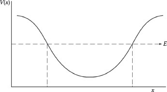
FIGURE 12.1
Static potential energy well V(x).

FIGURE 12.2
Potential energy well depicting a series of discrete energy levels E = 0, 1, 3, 4.

12.5.2  Semiconductor Emission

Going back to the time-independent Schrödinger’s equation

$\frac{{\partial }^2\text{ψ}(x)}{\partial x^2}-\frac{2m}{{\hslash }^2}(V(x)-E)\text{ψ}(x)=0$

(12.44)

and using the spatial component of the wave function as solution

$\text{ψ}(x)={\text{ψ}}_0{e}^{-ikx}$

(12.45)

leads directly to

$E=\frac{k^2{\hslash }^2}{2m}+V(x)$

(12.46)

This energy expression is the sum of kinetic and potential energy so that

$E_K+E_P=\frac{k^2{\hslash }^2}{2m}+V(x)$

(12.47)

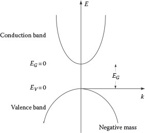
FIGURE 12.3
Conduction and valence bands according to E_K = ±(k²ħ²/2m).

and obviously

$E_K=\frac{k^2{\hslash }^2}{2m}$

(12.48)

The kinetic energy E_K as a function of k = 2π/λ is shown graphically in Figure 12.3.

The graph is a positive parabola for positive values of m and a negative parabola for negative values of m. In a semiconductor the positive parabola is known as the conduction band and the negative parabola is known as the valence band. The separation between the two bands is known as the band gap, E_G. If an electron is excited and transitions from the valence band to the conduction band, it is said to leave behind a vacancy or hole.

Electrons can transition from the bottom of the conduction band to the top of valence band by recombining with holes. In a material like gallium arsenide, the band gap is E_G ≈ 1.43 eV and the recombination emission occurs around 870 nm (Silfvast, 2008).

Under certain conditions radiation might also occur higher from the conduction band as suggested in Figure 12.4; however, that process is undermined by fast phonon relaxation.

12.5.3  Quantum Wells

Starting with a potential well as described by Silfvast (2008), V(x) = 0 for 0 < x < L, and V(x) = ∞ for x = 0 or x = L, as illustrated in Figure 12.5, then Equation 12.44

$\frac{{\partial }^2\text{ψ}(x)}{\partial x^2}-\frac{2m}{{\hslash }^2}(V(x)-E)\text{ψ}(x)=0$

FIGURE 12.4
Emission due to recombination transitions from the bottom of the conduction band to the top of the valence band.

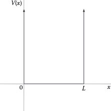
FIGURE 12.5
Potential well: V(x) = 0 for 0 < x < L, and V(x) = ∞ for x = 0 or x = L.

becomes

$\frac{{\partial }^2\text{ψ}(x)}{\partial x^2}-\frac{2m}{{\hslash }^2}E\text{ψ}(x)=0$

(12.49)

for 0 < x < L. This is a wave equation of the form

$\frac{d^2\text{ψ}(x)}{d{x}^2}+k_x^2\text{ψ}(x)=0$

(12.50)

with

$k_x^2=\frac{2m_c}{{\hslash }^2}E$

(12.51)

The solution to Equation 12.50 is

$\text{ψ}(x)=\sin k_{x}x$

(12.52)

Since ψ(x) = 0 at x = 0 or x = L, we have

$k_x=\frac{n\text{π}}{L}$

(12.53)

for n = 1, 2, 3…. Substituting Equation 12.53 into 12.51 leads to

$E=\frac{n^2{\text{π}}^2{\hslash }^2}{2m_c{L}^2}$

(12.54)

which should be labeled as E_n to account for the quantized nature of the energy, that is,

$E_n=\frac{n^2{\text{π}}^2{\hslash }^2}{2m_c{L}^2}$

(12.55)

This quantized energy E_n indicates a series of possible discrete energy levels above the lowest point of the conduction band so that the total energy above the valence band becomes (Silfvast, 2008)

$E=E_c+E_n$

(12.56)

12.5.4  Quantum Cascade Lasers

These lasers operate via transitions between quantized levels, within the conduction band, of multiple-quantum well structures. The carriers involved are electrons generated in an n-doped material. A single stage includes an injector and an active region. The electron is injected into the active region at n = 3, and the transition occurs down to n = 2 (see Figure 12.6). Following emission, the electron continues into the next injector region.

Practical devices include a series of such stages. From Equation 12.54, the energy difference between the two levels can be expressed as (Silfvast, 2008)

$\text{Δ}E=(3^2-2^2)\frac{{\text{π}}^2{\hslash }^2}{2m_c{L}^2}$

(12.57)

where L is the thickness of the well. Using ∆E = hν, it follows that the wave-length of emission is given by

$\text{λ}={(3^2-2^2)}^{-1}\frac{8m_{c}c{L}^2}{h}$

(12.58)

Quantum cascade lasers (Faist et al., 1994) are tunable sources emitting in the infrared from a few micrometers to beyond 20 Lm (see Appendix A).

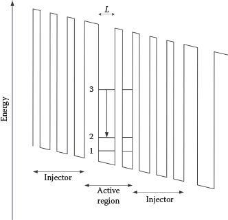
FIGURE 12.6
Simplified illustration of a multiple-quantum well structure relevant to quantum cascade lasers. An electron is injected from the “injector region” into the active region at n = 3. Thus a photon is emitted via the 3 → 2 transition. The electron continues to the next region where the process is repeated. By configuring a series of such stages, one electron can generate the emission of numerous photons.

12.5.5  Quantum Dots

Besides the multiple-quantum well configurations, other interesting semiconductor geometries include the quantum wire and the quantum dot. The quantum wire narrowly confines the electrons and holes in two directions (x, y). The quantum dot geometry severely confines the electrons in three dimensions (x, y, z). Under these circumstances the quantized energy can be expressed as

$E=E_c+\frac{k_x^2{\hslash }^2}{2m_c}+\frac{k_y^2{\hslash }^2}{2m_c}+\frac{k_x^2{\hslash }^2}{2m_c}$

(12.59)

where k_x, k_y, k_z are defined according to Equation 12.53.

The concept of quantum dot is not limited to semiconductor materials; it also applies to nanoparticle gain media and nanoparticle core–shell gain media. For instance, for nanoparticle core–shells the physics can be described with a Schrödinger’s equation of the form

${\nabla }^2\text{ψ}(r)-\frac{2m}{{\hslash }^2}(V(r)-E)\text{ψ}(r)=0$

(12.60)

with the potential V(r) defined by the core–shell geometry (Dong et al., 2013).

12.6  Introduction to the Hydrogen Equation

We have already seen that Schrödinger’s equation can be expressed as

$+i\hslash \frac{\partial \text{ψ}}{\partial t}=\widehat{H}\text{ψ}$

where the Hamiltonian is given by

$\widehat{H}=\left(-\frac{{\hslash }^2}{2m}\right){\nabla }^2+V(r)$

For an electron of mass m, under a potential V(r) described by

$V(r)=-\frac{e^2}{r}$

(12.61)

Schrödinger’s equation becomes

$+i\hslash \frac{\partial \text{ψ}}{\partial t}=-\frac{{\hslash }^2}{2m}{\nabla }^2\text{ψ}-\frac{e^2}{r}\text{ψ}$

(12.62)

Using a wave function of the form

$\text{ψ}(r,t)=e^{-iEt/\hslash }\text{ψ}(r)$

(12.63)

Equation 12.62 can be written as

$-\frac{{\hslash }^2}{2m}{\nabla }^2\text{ψ}(r)=\left(E+\frac{e^2}{r}\right)\text{ψ}(r)$

(12.64)

Using spherical polar coordinates

$\begin{array}{l}x=r\sin \text{θ}\text{cos}\text{ϕ}\hfill \\ y=r\sin \text{θ}\text{sin}\text{ϕ}\hfill \\ z=r\cos \text{θ}\hfill \end{array}$

(12.65)

the Laplacian

${\nabla }^2=\left(\frac{{\partial }^2}{\partial x^2}\right)+\left(\frac{{\partial }^2}{\partial y^2}\right)+\left(\frac{{\partial }^2}{\partial z^2}\right)$

operating on a function ϑ(r, θ, ϕ) can be written as (see, e.g., Flanders et al., 1970)

${\nabla }^2\vartheta (r,\text{θ},\text{ϕ})=r^{-1}\frac{{\partial }^2(rf)}{\partial r^2}+r^{-2}\left({\sin }^{-1}\text{θ}\frac{\partial }{\partial \text{θ}}\left(\sin \text{θ}\frac{\partial f}{\partial \text{θ}}\right)+{\sin }^{-2}\text{θ}\frac{{\partial }^{2}f}{\partial {\text{ϕ}}^2}\right)$

(12.66)

Thus, for a wave function ψ(r, θ, ϕ), Equation 12.64 can be expressed as

$r^{-1}\frac{{\partial }^2(r\text{ψ})}{\partial r^2}+r^{-2}\left({\sin }^{-1}\text{θ}\frac{\partial }{\partial \text{θ}}\left(\sin \text{θ}\frac{\partial \text{ψ}}{\partial \text{θ}}\right)+{\sin }^{-2}\text{θ}\frac{{\partial }^2\text{ψ}}{\partial {\text{ϕ}}^2}\right)=-\frac{2m}{{\hslash }^2}\left(E+\frac{e^2}{r}\right)\text{ψ}$

(12.67)

This is the Schrödinger’s equation applicable to the description of the hydrogen atom. The proper solution to this equation is mathematically rather lengthy and involves a number of tricks that are cleverly described by Feynman. Thus, the mathematically inclined is invited to read Feynman et al. (1965) on this subject. Also, the hydrogen atom is treated in various forms and depths by numerous textbooks on quantum mechanics (see, e.g., Schiff et al., 1968). Our main purpose here has been accomplished by introducing the type of notation necessary to describe the hydrogen atom and other small atoms.

In this regard, the Schrödinger’s equation has been use to describe small atoms such as hydrogen and helium in detail. However, as Feynman said: “in principle, Schrödinger’s equation is capable of explaining all atomic phenomena except those involving magnetism and relativity. It explains the energy levels of an atom and all the facts of chemical bonding” (Feynman et al., 1965). When Feynman first made this statement, this was only true in principle; however, the enormous advances in modern computational techniques have converted that statement into a reality.

Problems

12.1  Obtain Equation 12.5 by differentiating Equation 12.4 and substituting into Equation 12.3.

12.2  Show that Equation 12.15 follows from substitution of Equations 12.6 and 12.14 into Equation 12.11.

12.3  Use Equations 12.13 and 12.15 to obtain the Schrödinger’s equation in its well-known form, that is, Equation 12.18.

12.4  For a particle in a potential well V(x), assume that the wave function describing the state of the particle is given by ψ(x, t) = ϕ(x)ϑ(t). Given that

$\vartheta (t)=C{e}^{-i\text{ω}t}$

show that ϕ(x) and ϑ(t) satisfy the equation

$\frac{{\partial }^2\text{ψ}(x)}{\partial x^2}-\frac{2m}{{\hslash }^2}(V(x)-E)\text{ϕ}(x)=0$

12.5  Find the stationary solutions to the Schrödinger’s equation for the three regions (I, II, and III) defined in Figure 12.7. Hint: Starting from

$+i\hslash \frac{\partial \text{ψ}}{\partial t}=-\frac{{\hslash }^2}{2m}{\nabla }^2\text{ψ}+V\text{ψ}$

use a solution of the form

$\text{ψ}(x,t)=\text{ϕ}(x)\vartheta (t)$

to obtain

$\frac{{\partial }^2\text{ψ}(x)}{\partial x^2}-\frac{2m}{{\hslash }^2}(V(x)-E)\text{ϕ}(x)=0$

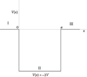
FIGURE 12.7
Potential well V(x) with regions I, II, and III, applicable to Problem 12.5. V(x) = 0 for x < 0, V(x) = − 2V for 0 ≤ x ≤ a, V(x) = 0 for x > a.

In region I, V(x) = 0, thus

$\begin{array}{c}\frac{{\partial }^2\text{ϕ}(x)}{\partial x^2}+\frac{2m}{{\hslash }^2}E\text{ϕ}(x)=0\\ \frac{{\partial }^2\text{ϕ}(x)}{\partial x^2}+k_1^2\text{ϕ}(x)=0\\ k_1={\left(\frac{2mE}{{\hslash }^2}\right)}^{1/2}\end{array}$

As already seen, this equation has a solution of the form

$\text{ϕ}(x)=C_1\sin k_{1}x$

12.6  Find the stationary solutions to the Schrödinger’s equation for the three regions (I, II, and III) defined in Figure 12.8.

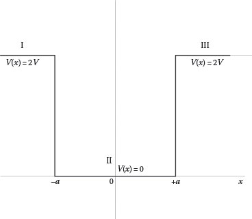
FIGURE 12.8
Potential well V(x) with regions I, II, and III, applicable to Problem 12.6. V(x) = 2V for x < −a, V(x) = 0 for a ≤ x ≤ −a, V(x) = 2V for x > a.

References

de Broglie, L. (1923). Waves and quanta. Nature 112, 540.

Dirac, P. A. M. (1978). The Principles of Quantum Mechanics, 4th edn. Oxford, London, U.K.

Dong, L., Sugunan, A., Hu, J., Zhou, S., Li, S., Popov, S., Toprak, M. S., Friberg, A. T., and Muhammed, M. (2013). Photoluminescence from quasi-type-II spherical CdSe-CdS core-shell quantum dots. Appl. Opt. 52, 105–109.

Faist, J., Capasso, F., Sivco, D. L., Sirtori, C., Hutchinson, A. L., and Cho A. Y. (1994). Quantum cascade laser. Science 264, 553–556.

Feynman, R. P., Leighton, R. B., and Sands, M. (1965). The Feynman Lectures on Physics, Vol. III. Addison-Wesley, Reading, MA.

Flanders, H., Korfhage, R. R., and Price, J. J. (1970). Calculus. Academic, New York.

Haken, H. (1981). Light. North-Holland, Amsterdam, the Netherlands.

Herzberg, G. (1950). Spectra of Diatomic Molecules. Van Nostrand Reinhold, New York.

Hooker, S. and Webb, E. (2010). Laser Physics. Oxford University, Oxford, U.K.

Planck, M. (1901). Ueber das gesetz der energieverteilung im normalspectrum. Ann. Phys. 309(3), 553–563.

Saleh, B. E. A. and Teich, M. C. (1991). Fundamentals of Photonics, Wiley, New York.

Schiff, L. I. (1968). Quantum Mechanics. McGraw-Hill, New York.

Schrödinger, E. (1926). An undulatory theory of the mechanics of atoms and molecules. Phys. Rev. 28, 1049–1070.

Silfvast, W. T. (2008). Laser Fundamentals, 2nd edn. Cambridge University, Cambridge, U.K.