Chapter 23

Dirichlet process models

The Dirichlet process is an infinite-dimensional generalization of the Dirichlet distribution that can be used to set a prior on unknown distributions. Furthermore, these unknown densities can be used to extend finite component mixture models to infinite component mixture models.

23.1   Bayesian histograms

We start in this section and the next with the relatively simple setting in which y_i f and the goal is to obtain a Bayes estimate of the density f. The histogram is often (also in this book) used as a simple form of density estimate. In this section we develop a flexible parametric version of the histogram that helps to motivate the fully nonparametric Bayesian density estimation of the following section. The remainder of the chapter shows how the Dirichlet process can be applied beyond density estimation.

Assume we have prespecified knots to define our histogram estimate, with ξ₀ < ξ₁ < ··· < ξ_k-1 < ξ_k and y_i [ξ₀, ξ_k]. A probability model for the density that is analogous to the histogram is as follows:

with π = (π₁, …, π_k) an unknown probability vector. We complete a Bayes specification with a prior distribution for the probabilities. Assume a Dirichlet(a₁, …, a_k) prior distribution for π,

The hyperparameter vector can be re-expressed as a = απ₀, where

is the prior mean and α is a scale that is often interpreted as a prior sample size.

The posterior distribution of π is then calculated as

where n_h = σ_i 1_{ξh-1<yi≤ξh} is the number of observations falling in the hth histogram bin.

To illustrate the Bayesian histogram method, we simulated data from the mixture,

with n = 100 samples drawn from this density. Assuming data between [0, 1] and choosing 10 equally spaced knots, we applied the Bayesian histogram approach and plotted the true density and simulations from the posterior distribution of the histogram obtained from this procedure.

The Bayesian histogram estimator does an adequate job approximating the true density, but the results are sensitive to the number and locations of knots. However, an appealing property of the Bayesian histogram approach is that implementation is easy since we have conjugacy and the posterior can be calculated analytically. In addition, the approach allows prior information to be included and allows easy production of interval estimates, and hence has some practical advantages over classical histogram estimators. To improve performance a prior can be placed on the numbers and locations of knots, with reversible jump MCMC (see Section 12.3) used for computation, but such an approach is computationally demanding. In addition, even averaging over random knots will tend to introduce artifactual bumps in the density estimate. The Dirichlet prior distribution is perhaps not the best choice due to the lack of smoothing across adjacent bins, but it does have the advantage of conjugacy and simplicity in interpretation of the hyperparameters.

23.2   Dirichlet process prior distributions

Definition and basic properties

Motivated by the simplicity of the Bayesian histogram approach with a Dirichlet prior, one wonders whether we can somehow bypass the need to explicitly specify bins. This would also facilitate extensions to multivariate cases in which there is an explosion of the number of bins that would be needed. With this thought in mind, suppose the sample space is Ω, partitioned into measurable subsets B₁, …, B_k. If Ω = , then B₁, …, B_k are simply non-overlapping intervals partitioning the real line into a finite number of bins.

Let P denote the unknown probability measure over (Ω, ), with the collection of all possible subsets of the sample space Ω. The probability measure will assign probabilities to these subsets (bins), with the probabilities allocated to a set of bins B₁, …, B_k partitioning Ω being

If P is a random probability measure (RPM), then these bin probabilities are random variables. A simple conjugate prior for the bin probabilities corresponds to the Dirichlet distribution. For example, we could let

where P₀ is a base probability measure providing an initial guess at P, and α is a prior concentration parameter controlling the degree of shrinkage of P toward P₀.

Prior (23.1) is essentially a Bayesian histogram model closely related to that described in the previous section. However, the difference is that (23.1) only specifies that bin B_k is assigned probability P(B_k) and does not specify how probability mass is distributed across the bin B_k. Hence, for a fixed partition B₁, …, B_k, (23.1) does not induce a fully specified prior for the random probability measure P. The idea is to eliminate sensitivity to the choice of partition B₁,…, B_k and induce a fully specified prior on P through assuming (23.1) holds for all possible partitions B₁, …, B_k and all k.

For this specification to be coherent, there must exist a random probability measure P such that the probabilities assigned to any measurable partition B₁, …, B_k by P is Dirichlet(αP₀(B₁), …, αP₀(B_k)). The existence of such a P can be shown by verifying certain consistency conditions, and the resulting random probability measure P is referred to as a Dirichlet process. Then, as a concise notation to indicate that a probability measure P on (Ω, ) is assigned a Dirichlet process (DP) prior, let P ~ DP(αP₀), where α > 0 is a scalar precision parameter and P₀ is a baseline probability measure also on (óM, ). This baseline P₀ is commonly chosen to correspond to a parametric model such as a Gaussian.

The definition of the Dirichlet process and properties of the Dirichlet distribution imply,

so that the marginal random probability assigned to any subset B of the support is simply beta distributed. It follows directly that the prior mean has the form

so that the prior for P is centered on P₀. In addition, the prior variance is

so that α is a precision parameter controlling the variance.

Hence, the Dirichlet process is appealing in having a simple specification arising from a model similar to a random histogram but without the dependence on the bins, while also having simple and intuitive forms for the prior mean and variance. The prior can be centered on a parametric model for the distribution of the data through the choice of P₀, while allowing α to control uncertainty in this choice. Moreover, it can be shown that the support of the DP contains all probability measures whose support is contained in the support of the baseline probability measure P₀.

The DP prior distribution also has a conjugacy property which makes inferences straightforward. To demonstrate this, first let y_i P, for i = 1, …, n and P ~ DP(αP₀), where we follow common convention in using P to denote both the probability measure and its corresponding distribution. Then, from (23.1) and conjugacy properties of the finite Dirichlet distribution, for any measurable partition B₁, …, B_k, we have

From this and the above development, it is straightforward to obtain

The updated precision parameter is α + n, so that α is in some sense a prior sample size. The posterior expectation of P is defined as

Hence, the Bayes estimator of P under squared error loss is the empirical measure with equal masses at the data points shrunk toward the base measure. It is clear that as the sample size increases, the Bayesian estimate of the distribution function under the Dirichlet process prior will converge to the empirical distribution function.

In addition, in the limit as the precision parameter α approaches 0, so that we in some sense have a noninformative prior distribution, the posterior distribution is

This limiting posterior distribution is sometimes known as the Bayesian bootstrap. Samples from the Bayesian bootstrap correspond to discrete distributions supported at the observed data points with Dirichlet distributed weights. Compared with the classical bootstrap, the Bayesian bootstrap leads to smoothing of the weights.

Even with these many appealing properties, the Dirichlet process prior distribution has some important drawbacks. Firstly, there is a lack of smoothness apparent in (23.2). Ideally, one would not simply take a weighted average of the base measure and the empirical measure with masses at the observed data points, but would allow smooth deviations from the base measure. Smoothness would imply dependence between P(B₁) and P(B₂) for adjacent bins B₁ and B₂. However, the DP actually induces negative correlation between P(B₁) and P(B₂) for any two disjoint sets B₁ and B₂, with no account for the distance between these sets. An even more important concern for density estimation is that realizations from the DP are discrete distributions. Hence, P ~ DP(αP₀) implies that P will be atomic having nonzero weights only on a set of atoms and will not have a continuous density on the real line.

Despite these drawbacks the DP has been useful in developing flexible models for a wide variety of problems. Before demonstrating some of the applications we introduce an alternative characterization of the Dirichlet process.

Stick-breaking construction

The above specification of the Dirichlet process does not provide an intuition for what realizations P ~ DP(αP₀) actually look like, since the DP prior was defined indirectly through the marginal probabilities allocated to finite partitions. However, there is a direct constructive representation of the Dirichlet process, which is referred to as the stick-breaking representation, which is useful in obtaining further insight into properties of the DP and as a stepping stone for generalizations.

The stick-breaking representation allows us to induce P ~ DP(αP₀) by letting

where δ_θ denotes a degenerate distribution with all its mass at θ, the atoms (θ_h)_h=1^∞ are generated independently from the base distribution P₀, π_h is the probability mass at atom θ_h, and these probability masses are generated from a so-called stick-breaking process that guarantees that the weights sum to 1.

To describe the stick-breaking process, we start with a stick of unit length representing the total probability to be allocated to all the atoms. We initially break off a random piece of length V₁, with the length generated from a Beta(1, α) distribution, and allocate this π₁ = V₁ probability weight to the randomly generated first atom θ₁ ~ P₀. There is then 1 - V₁ of the stick remaining to be allocated to the other atoms. We break off a proportion V₂ ~ Beta(1, α) of the 1 - V₁ stick and allocate the probability π₂ = V₂(1 - V₁) to the second atom θ₂ ~ P₀. As we proceed, the stick gets shorter and shorter so that the lengths allocated to the higher indexed atoms decrease stochastically, with the rate of decrease depending on the DP precision parameter α. Because E(V_h) = 1/1+α, values of α close to zero lead to high weight on the first couple atoms, with the remaining atoms being assigned small probabilities.

Figure 23.1  Samples from the stick-breaking representation of the Dirichlet process with different settings of the precision parameter α.

Figure 23.1 shows realizations of the stick-breaking process for P₀ corresponding to a standard normal distribution and different values of α. From this figure it is apparent that the DP is not appropriate as a direct prior on the distribution of the data, particularly if the data are continuous. For continuous data, each new subject requires a new atom so that a large value of α is required, implying weight close to zero on each atom and hence a small probability of ties in the realizations from P. In the limit as α → ∞, one obtains y_i ~ P₀, and hence for large α and no ties in the observations, the DP prior effectively models the data are drawn from the parametric base distribution.

23.3   Dirichlet process mixtures

Specification and Polya urns

The failure of the DP prior distribution as a direct model for the distribution of the data does not imply that it is not useful in applications. Instead, the DP is more appropriately used as a prior for an unknown mixture distribution. Focusing again on the density estimation case for simplicity, a general kernel mixture model for the density can be specified as

where κ(·θ) is a kernel, with θ including location and possibly scale parameters, and P is a mixing measure. In the special case in which P is treated as discrete with masses at a finite number of k atoms, one obtains a finite mixture model as discussed in Chapter 22.

In a infinite kernel mixture model, one chooses a prior P ~ π for the unknown mixing measure , where denotes the space of all probability measures on (Ω, ) and π denotes a prior over this space. The prior for the mixing measure induces a prior on the density f(y) through the integral mapping in (23.3). If π is chosen to correspond to a DP prior, then one obtains a DP mixture model. From (23.2) and (23.3), a DP prior on P leads to

where π =~ stick(α) is a shorthand notation to denote that the probability weights are sampled from a DP stick-breaking process with parameter α, and with θ_h ~ P₀ independently for h = 1, …, ∞.

Expression (23.4) resembles the finite mixture models considered in Chapter 22, but with the important difference that the number of mixture components (latent subpopulations) is set to infinity. However, this does not imply that infinitely many components are occupied by the subjects in the sample; rather, the model allows flexibility by introducing new mixture components as subjects are added. Consider the hierarchical specification in which

This formulation is equivalent to sampling y_i from the infinite mixture model in (23.4). A key question is how to conduct posterior computation under this DP mixture (DPM)? This initially seems problematic in that the mixing measure P is characterized by infinitely many parameters, as is apparent in (23.2), and we no longer have joint conjugacy in which the posterior of P given yⁿ = (y₁, …, y_n) has a simple form.

A clever way around this problem is to marginalize out P to obtain an induced prior distribution on the subject-specific parameters θⁿ = (θ₁, …, θ_n). In particular, marginalizing out P, we obtain the Polya urn predictive rule,

This conditional prior distribution consists of a mixture of the base measure P₀ and probability masses at the previous subject’s parameter values.

A Chinese restaurant process metaphor is commonly used in describing the Polya urn scheme. Consider a restaurant with infinitely many tables. The first customer sits at a table with dish θ₁^*. The second customer sits at the first table with probability α/1+α or a new table with probability 1/1+α. This process continues with the ith customer sitting at an occupied table with probability proportional to the number of previous customers at that table and sitting at a new table with probability proportional to α. Each occupied table in the (infinite) restaurant represents a different cluster of subjects, with new clusters added at a rate proportional to α log n in the asymptotic limit. The number of clusters depends (probabilistically) on the number of subjects n with new clusters introduced as needed as additional subjects are added to the sample. This makes more sense in typical applications than finite mixture models in which k does not depend on n and can be thought of as a formal procedure mimicking the good practice, when fitting a finite mixture model, of manually adding new mixture components as necessary to fit the data.

The simple form for the conditional distribution in (23.5) leads to a useful idea for posterior computation and prediction. From exchangeability of the subjects i = 1, …, n, one can obtain the conditional prior distribution for as

where , are the unique values of θ^(-i), and .

Updating the full conditional prior (23.6) with the data, one obtains a conditional posterior distribution for θ_i having the same form but with updated weights on the components and updated P₀, as long as P₀ is conjugate to the kernel κ. For example, this occurs when κ(·θ) is a normal kernel, with θ = (μ, ) the mean and precision and P₀ a normal-gamma prior distribution. Potentially, one can update the θ_i’s one at a time from these full conditional posterior distributions in implementing Gibbs sampling. However, this approach tends to have poor mixing.

An alternative marginal Gibbs sampler, which instead separately updates the allocation of subjects to clusters and the cluster-specific parameters, proceeds as follows. Let θ^* = (θ₁^*, …, θ_k^*) denote the unique values of θ and let S_i = c if θ_i = θ_c^* so that S_i denotes allocation of subject i to a cluster. The Gibbs sampler alternates between

1.  Update the allocation S by sampling from the multinomial conditional posterior with

If S_i = k^(-i) + 1, then subject i is allocated to a singleton cluster.

2.  Update the unique values θ^* by sampling from

which is simply the posterior distribution under the parametric model that assigns prior distribution P₀ to the parameters θ_h^* and then updates this prior with the likelihood for those subjects in cluster h.

When P₀ is conjugate to the kernel κ, the integral in step 1 can be calculated analytically and the conditional posterior in step 2 has the same parametric form as P₀ except with updated parameters. For example, when the kernel is Gaussian, with θ the mean and variance and P₀ a conjugate normal-inverse-gamma prior, the conditional distribution of θ_c^* has the same normal-inverse-gamma form described in Chapter 22 in the finite mixture case. There are modifications available to accommodate nonconjugate cases as well.

In step 1 of the above Gibbs sampler, either the ith subject is allocated to an existing cluster occupied by one of the other subjects in the sample or the subject is allocated to a new cluster. The conditional posterior probability of allocation to a new cluster is proportional to the DP precision parameter α multiplied by the marginal likelihood for the ith subject’s data, obtained in integrating the likelihood κ(y_iθ) over the prior θ ~ P₀. If α is close to zero or this marginal likelihood is small relative to the likelihoods for the ith subject’s data given allocation to one of the occupied clusters, then subject i will tend to be allocated to an existing cluster. Hence, both α and P₀ play important roles in controlling the posterior distribution over clusterings. As α decreases, there is an increasing tendency to cluster subjects, with a parametric model y_i ~ K(θ) for a common θ obtained in the limit as α → 0. In practice, it is common to either set α = 1 to favor allocation to few clusters or to choose a gamma hyperprior for α to allow greater data-adaptivity, with an additional MCMC step included to update α.

Somewhat more subtle, and often overlooked, is the role of P₀ in controlling clustering behavior. One may naively try a high variance P₀ to express ignorance about the prior distribution of likely locations for the different kernels. However, similarly as discussed in Section 7.4, a flat prior for P₀ can turn out to make strong assumptions, in this case effectively placing a heavy penalty on the introduction of new clusters. This is because as the variance of P₀ becomes high, the marginal likelihood will decrease, since the prior P₀ places small probability in a region of plausible θ values in such cases. In the limit as the variance of P₀ → ∞, the posterior will behave as if the likelihood is y_i ~ K(θ) with a common θ for all individuals. In practice, we recommended constructing an informative P₀ placing high probability on introducing clusters near the support of the data; this can be facilitated by standardizing the data in advance of the analysis. Refer to the relevant discussion in Chapter 22.

This Gibbs sampler for Dirichlet process models closely resembles the Gibbs sampler for finite mixtures, with the main difference being that we marginalize out the weights π on the different clusters and allow the number of clusters to vary across the samples. The number of mixture components k represented in the sample of n subjects is treated as unknown, and we obtain samples from the posterior of k automatically without needing a reversible jump MCMC algorithm. From the Gibbs samples, we can also estimate the predictive density of y_n+1 using averaged over posterior simulations. The simplicity of this Gibbs sampler and the ability to bypass the issue of selection of k by embedding in an infinite mixture model, which automatically introduces new components at a slow rate as needed when additional subjects are added to the sample, are major reasons for the large applied success of Dirichlet process mixture models.

The Gibbs sampler for finite mixture models introduced in Chapter 22 provides an approximation to a DP mixture model with P ~ DP(αP₀) as long as the mixture component-specific parameters are drawn iid a priori from P₀ and the prior on the weights is π ~ Dirichlet(α/k, …, α/k). The approximation improves with k and in practice one can set k equal to a conservative upper bound on the number of occupied clusters in the sample (k = 25 or 50 can work well). Indeed, we refer the reader to the discussions in Chapter 22 pertaining to the issues that arise in finite mixture modeling, as essentially the same issues arise in infinite discrete mixtures, such as DPMs, and the same solutions apply.

Blocked Gibbs sampler

By marginalizing out the random probability measure P, we give up the ability to conduct inferences on P. By having approaches that avoid marginalization, we open the door to generalizations of DPMs for which marginalization is not possible analytically. One approach for avoiding marginalization is to rely on the construction in (23.4). Because the stick-breaking construction orders the mixture components so that the weights are stochastically decreasing in the index h, for a sufficiently high index N, we will have that σ_N+1^∞ π_h has a distribution concentrated near zero. Hence, we can obtain an accurate approximation by letting V_N = 1 in the stick-breaking process so that π_h = 0 for h = N+1, …, ∞, with N chosen to be sufficiently large. In practice, N = 25 or 50 is commonly chosen as a default, with N providing an upper bound on the number of clusters in the n subjects in the sample. We have rarely seen a need for more than 10 or 15 clusters to accurately fit the unknown density.

The truncation approximation to the DP leads to a straightforward MCMC algorithm for posterior computation, and represents an alternative to the finite Dirichlet approximation described in Chapter 22. It is not clear which of these approaches leads to more efficient posterior computation, though the exchangeability of the components in the finite Dirichlet approximation conveys some advantages in terms of mixing. Using the stick-breaking truncation, the following blocked Gibbs sampler can be used:

1.  Update S_i {1, …, N} by multinomial sampling with

where denotes that subject i is allocated to cluster c.

2.  Update the stick-breaking weight V_c, c = 1, …, N-1, from Beta .

3.  Update θ_c^*, c = 1, …, N, exactly as in the finite mixture model, with the parameters for unoccupied clusters with n_c = 0 sampled from the prior P₀.

This algorithm involves simple sampling steps and is straightforward to implement. In order to estimate the density f(y) one can follow the approach of monitoring at each iteration over a dense grid of y values (for example, an equally spaced grid of 100 values ranging from the minimum of the observed y’s minus a small buffer to the maximum of the observed y’s plus a small buffer). Based on these samples, we can compute posterior inferences.

When running the algorithm, it is good practice to monitor S_max = max(S₁, …, S_n) to verify that the maximum occupied component index has a low probability of being close to the upper bound of N. Otherwise, the upper bound should be increased. Convergence should be monitored on the sampled f(y) values and not to the mixture component-specific parameters. As discussed in Chapter 22, label ambiguity problems often lead to poor mixing of the component-specific parameters, but this may not impact convergence and mixing of the induced density of interest.

Gibbs sampling algorithms that rely on stick-breaking representations have performed well in our experience. But in some cases, all of the above algorithms can encounter slow mixing that arises due to the multimodal nature of the posterior in which it can be difficult to move rapidly between different clusterings. This mixing problem can be partly addressed by incorporating label switching moves and there is also a literature on split-merge algorithms designed for more rapid exploration of the distribution of cluster allocations.

Hyperprior distribution

The DP precision parameter α plays a key role in controlling the prior on the number of clusters, and there are a number of possible strategies in terms of specifying α. One can fix α at a small value to favor allocation to few clusters relative to the sample size, with a commonly used default value corresponding to α = 1. This implies that, in the prior distribution, two randomly selected individuals have a 50–50 chance of belonging to the same cluster. Alternatively, one can allow the data to inform about the appropriate value of α by choosing a hyperprior, such as α ~ Gamma(a_α, b_α), and then updating α during the MCMC analysis. For the blocked Gibbs sampler, the gamma hyperprior is conditionally conjugate with the resulting conditional posterior being

Hence, sampling from this conditional can be included as an additional step in the algorithm described in the previous subsection.

In our experience, the data tend to be informative about the precision parameter α of the Dirichlet process, and hence there is substantial Bayesian learning, with a high variance prior often resulting in a concentrated, low-variance posterior. It may seem counterintuitive that the data can inform strongly about the number of clusters through the hyperparameter α given that maximum likelihood estimation leads to overfitting, with more clusters resulting in a higher maximized likelihood. However, the Bayesian approach favors clusterings and values of α that result in a high marginal likelihood. If individuals are allocated to many different clusters, the effective number of parameters in the likelihood is increased, and we then integrate across a larger space in calculating the marginal likelihood. This induces an intrinsic penalty that favors allocation to few clusters that are really needed to fit the data; there is no tendency for overfitting.

The more difficult and subtle issue is choice of the base measure P₀. Often the base measure is chosen for computational convenience to be conjugate. However, even in conjugate parametric families such as normal-gamma, we can potentially improve flexibility by placing hyperparameters on the parameters in P₀. P₀ can be thought of as inducing the prior for the cluster locations. If these locations are too spread out, because P₀ has high variance, then the penalty in the marginal likelihood for allocating individuals to different clusters will be large, and the tendency will be to overly favor allocation to a single cluster.

It is crucial to consider the measurement scale of the data in choosing P₀. The variance of P₀ is only meaningful relative to the scale of the data. A common approach is to standardize the data y and then choose P₀ to be centered at zero with close to unit variance. If we set unit variance and do not standardize, then how flat P₀ is depends on the unit of measurement in the data—if we change from inches to miles, we may get completely different results.

Figure 23.2  Histogram of the number of implantations per pregnant mouse in the control group (black line) and posterior mean of Pr(y = j) assuming a Dirichlet process prior on the distribution of the number of implants with α = 1, 5 (gray and black dotted lines, respectively) and base measure P₀ = Poisson().

Figure 23.3  Histogram of a subsample of size 10 from the control group on implantation in mice (black line) and posterior mean of Pr(y = j) assuming a DP prior on the distribution of the number of implants with α = 1, 5 (gray and black dotted lines, respectively) and base measure P₀ = Poisson().

In this case, we can easily work out the steps involved in the blocked Gibbs sampler.

1.  Update S_i {1,…, N} by multinomial sampling with

where S_i = c if θ_i = θ_c^* denotes that subject i is allocated to cluster h.

2.   Update the stick-breaking weight V_c, c = 1,…, N - 1, from

3.  Update θ_h^*, h = 1, …, N, from its conditional posterior,

with n_c = σ_i=1ⁿ 1_Si=c, the size of the c-th cluster.

A conservative upper bound of N = n can be used for the truncation level.

Although a Dirichlet process mixture of Poissons is the obvious choice and leads to simple computation, there is a lurking problem with this approach, which is a common issue in hierarchical Poisson models in general. In particular, the Poisson kernel is inflexible in that it restricts the mean and variance to be equal. In using a mixture of Poissons, such as the DPM in (23.7), one can only increase the variance relative to the mean. Hence, mixtures of Poissons are only appropriate for modeling overdispersed count distributions and produce poor results in the toxicology data on implantations. In particular, the estimated dose group-specific distributions of the number of implants under the DPM of Poissons exhibit substantially larger variance than the empirical distributions, suggesting a poor fit.

For continuous data, Gaussian kernels are routinely used and do not have this pitfall in having separate parameters for the mean and variance. Gaussians are easily modified to the count case by relying on rounding. In particular, let

with h(·) a rounding function that has for , and . For this rounded Gaussian kernel, we can derive a simple blocked Gibbs sampler, which has the following steps.

1.  Update S_i {1, …, N} by multinomial sampling with

where is the normal cumulative distribution function with location μ and precision τ.

2.  Update stick-breaking weight V_h, h = 1, …, N - 1, from

3.  Generate each y_i^* from the full conditional posterior

4.  Update θ_c^* = (μ_c^*, τ_c^*), c = 1, …, N, from its conditional posterior,

with .

Essentially, we just impute the latent y_i^* within the third step of the Gibbs sampler and otherwise proceed as if we were modeling the data using a DPM location-scale mixture of Gaussians. In fact, the above steps can also be used for Bayesian density estimation of continuous densities in which the observed data are y_i^* and we have no need for step 3.

We repeated our analysis of the toxicology data on implantations using the DPM of rounded Gaussians approach, and obtained an excellent fit to the data, improving on the DPM of Poissons result. The empirical cumulative distribution functions are entirely enclosed within pointwise 95% credible intervals. To conduct inferences on changes in the distribution of the number of implants with dose, we estimated summaries of the posterior distributions for changes in each percentile between the control group and each of the exposed groups. Negative changes for an exposed group relative to control suggest an adverse impact of dose. The estimated posterior probabilities of a negative average change across the percentiles was 0.72 in the 750 mg/kg group, 0.99 in the 1500 mg/kg group, and 0.94 in the 3000 mg/kg group. Hence, there was substantial evidence of a stochastic decrease in the number of implants in the higher two dose groups relative to control.

23.4   Beyond density estimation

Nonparametric residual distributions

Density estimation has been used to this point primarily to simplify the exposition of a difficult topic. The real attraction of Dirichlet process mixture (DPM) models is that they can be used much more broadly for relaxing parametric assumptions in hierarchical models. This section is meant to give a flavor of some of the possibilities without being comprehensive. First, consider the linear regression setting with a nonparametric error distribution:

where is a vector of predictors and _i is an error term with distribution f. The assumption of linearity in the mean is easily relaxed as discussed earlier. Here, we consider the problem of relaxing the assumption that f, the distribution of errors, has a parametric form.

In Chapter 17 we considered the t model as a way to downweight the influence of outliers. This is easily accomplished computationally by expressing the t_ν distribution as a scale mixture of normals by letting _i ~ N(0, _i^-1 σ²), with _i ~ Gamma ~ (ν/2, ν/2). Although the t distribution may be preferred over the normal due to its heavy tails, it still has a restrictive shape and we could instead model f nonparametrically using a DP scale mixture of normals:

where P₀ is chosen to correspond to Gamma(ν/2, ν/2) to center the prior for f on a t distribution, while allowing more flexibility. The resulting prior for f is flexible but is still restricted to be unimodal and symmetric about zero.

An alternative which removes the unimodality and symmetry constraints is to use a location mixture of Gaussians for f. Removing the intercept from the X_iβ term and allowing f to have an unknown mean, let

with P₀ chosen as N(0, τ^-1). The computations for density estimation can be easily adapted to include steps for updating the regression coefficients β and then replacing y_i with y_i - X_iβ in the previous steps.

Nonparametric models for parameters that vary by group

In Chapter 15 we considered hierarchical linear models with varying coefficients. Uncertainty about the distribution of the coefficients can be taken into account by placing DP or DPM priors on their distributions. As a simple illustration, consider the one-factor Anova model,

with y_i = (y_i1, …, y_{i, ni}) a vector of repeated measurements for item i, μ_i a subject-specific mean, and _ij an observation-specific residual. Typical parametric models would let f correspond to a N(μ, ψ^-1) density, while letting g ≡ N(0, σ²).

To allow more flexibility in characterizing variability among subjects, we can instead let

where P is the unknown distribution of the varying parameters and for simplicity we model the residual density g as N(0, σ²). Placing a DP prior on the distribution induces a latent class model in which the subjects are grouped into an unknown number of clusters, with

where S_i {1, …, ∞} is a latent class index, and π_h is the probability of allocation to latent class h, with these probabilities following the stick-breaking form as in (23.2). As for finite latent class models, this formulation assumes that the distribution of the varying parameters is discrete so that different subjects can have identical values of the parameters. This may be useful as a simplifying assumption and the posterior means will be different for every subject, since the clustering is soft and probabilistic, with the posterior means of μ_i obtained averaging across the posterior distribution on the cluster allocation.

There are some practical questions that arise in considering nonparametric hierarchical models such as (23.10). The first is whether the data contain information to allow nonparametric estimation of P given that the modeled parameters μ_i are not observed directly for any of the subjects. The answer to this question and the interpretation of the resulting estimate depends on the number of observations per subject. Suppose initially that n_i = 1 for all subjects. In this case, we do not have any information in the data to distinguish variability among subjects from variability among measurements within a subject. However, under the assumption of normality of the residual density g, we still have substantial information in the data about P in that P accommodates lack of fit of the normal residual distribution. In the general case in which n_i ≥ 1 and normal g is assumed, P has a dual role in allowing for lack of fit of the normal distribution for the residuals and systematic variability among subjects. When there are many observations per subject, that later role dominates, but when n_i is small interpretation of P needs to take into account the dual roles.

One natural possibility for removing this confounding is to also model g using a Dirichlet process mixture of Gaussians. In this case, the data contain less information about the distribution, and accurate estimation may require a dataset with many observations per item and many items. In the case in which the distribution of the parameters and the residual distribution are both unknown, an identifiability issue does arise in that it is difficult in nonparametric Bayes models to restrict the mean of the distribution to be zero. However, one can run the MCMC analysis for an overparameterized model without restrictions on the means and then post-process to estimate the overall mean and mean-centered parameters and residual densities.

Functional data analysis

In Chapter 21 we discussed Gaussian processes for functional data analysis, where responses and predictors for a subject are not modeled as scalar or vector-valued random variables but instead as random functions defined at infinitely many points. Here we consider a basis function expansion related to the approaches considered in Chapter 20.

Let y_i = (y_i1, …, y_ini) denote the observations on function f_i for subject i, where y_ij is an observation at point t_ij, with t_ij τ. Allowing for measurement errors in observations of a smooth trajectory, let

and

where b = {b_l}_h=1^H is a collection of basis functions and θ_i is a vector of subject-specific basis coefficients. Here, we are assuming a common collection of potential basis functions, but by allowing elements of the θ_i coefficient vectors to be zero or close to zero, we can discard unnecessary basis functions and even accommodate subject-specific basis function selection. In many applications, it is necessary to allow different subjects to have a different basis for sufficient flexibility. By using a common dictionary of bases across subjects, we allow a common backbone from which a hierarchical model for borrowing information can be built.

To borrow information across subjects and model the variability in the individual functions, let

where the H-dimensional distribution P must be specified or modeled. Potentially, we can consider a parametric family in which P = N_H(θ, Ω), with the resulting mean function then corresponding to , where b(t) = (b₁(t), …, b_H(t)). This mean function provides a population-averaged curve. In addition, the hierarchical covariance matrix Ω characterizes heterogeneity among the subjects in their functions. There are several practical issues that arise with this parametric hierarchical model. Firstly, the number of basis functions p is typically moderate to large, and hence Ω will have many parameters and it can be difficult to reliably estimate all these parameters. In addition, there is no allowance for basis function selection through shrinking the basis coefficients to zero. Although one could potentially choose a prior for Ω that allows diagonal elements close to zero, this would discard the corresponding basis functions for all subjects and does not accommodate subject-specific selection. Finally, the normality assumption for the varying parameters implies a restrictive type of variability across subjects; for example, it cannot accommodate sub-populations of subjects having different functions and outlying functions.

An alternative is to use a Dirichlet process prior, . This will induce functional clustering with

All individuals within cluster c will have , with the basis coefficients characterizing the cluster c function being θ_c^* = (θ_c1^*, …, θ_cH^*). By choosing an appropriate base measure P₀ within the functional DP, one can allow the basis functions to differ across the clusters and hence allow individual-specific basis selection through cluster-specific basis selection.

There are two good possibilities in this regard. Firstly, one can let , with P_0h specified to have a variable selection-type mixture form: possibly with ψ_h ~ Gamma(ν/2, ν/2) to induce a heavy-tailed t prior for the nonzero basis coefficients. In sampling the cluster-specific basis coefficients from this prior, θ_ch^* ~ P_0h independently for h = 1, …, H, a subset of the elements of θ_c^* will be exactly equal to 0, with this subset varying across the different functional clusters. By letting π_0h ~ Beta(a, b), one can allow uncertainty in the prior probability of exclusion of the h-th basis function, while borrowing information across functional clusters in learning about which basis functions are needed overall.

This approach leads to a straightforward Gibbs sampler, incorporating minor modifications to the blocked Gibbs sampling or finite Dirichlet approximation algorithms described above. After allocating subjects to clusters, we can update θ_ch^* by direct sampling from its full conditional distribution, which will have a mixture form consisting of a point mass at zero and a normal distribution. This has a similar form to that described in Chapter 20 for nonparametric regression with basis selection. Each pass through the Gibbs updating steps will vary the allocation of subjects to functional clusters and the basis functions selected to characterize the functional trajectories. Based on the resulting posterior samples, we can obtain model-averaged estimates of the functions specific to each subject.

Although this approach tends to work well in practice, the one-at-a-time updates of the θ_ch^*s specific to each cluster and basis function can lead to a high computational burden for each iteration of each Gibbs sweep as well as slow mixing of the chains. An alternative that leads to similar estimation performance in practice, while simplifying and substantially speeding up posterior computation, is to use a heavy-tailed shrinkage prior in place of the variable selection mixture prior. In particular, one simple choice is with ν chosen to be small; for example, ν = 1 provides a default that leads to a Cauchy marginal prior for the basis coefficients. Under this approach, the basis coefficient vectors θ_c^* can be updated in a block from multivariate normal full conditional posterior distributions. This block updating can accelerate mixing substantially. Although this approach does not formally allow for basis selection in that none of the coefficients will be exactly zero, the prior is concentrated at zero with heavy tails and hence allows coefficients that are close to zero. For small basis coefficients, the corresponding basis functions are effectively excluded and in practice it is impossible to distinguish small nonzero coefficients from coefficients that are exactly zero. In most applications, it can be argued that coefficients will not be exactly zero in any case.

23.5   Hierarchical dependence

In the previous sections we discussed Dirichlet process mixture models for a single unknown distribution. This unknown distribution can be the distribution of the data directly or some component of a hierarchical Bayesian model. To build rich semiparametric hierarchical models, one may potentially incorporate several DPs, set to be independent in the prior distribution. This approach was implemented in the toxicology data analysis in the previous section. However, there are clear limits to this strategy and in many settings it is appealing to use priors that favor dependence in unknown distributions. To motivate the need for such generalizations, we start by describing an application in which such flexibility is warranted.

Figure 23.4  Histograms and kernel-smoothed density estimates of DNA damage across cells in each hydrogen peroxide dose group in the genotoxicity example.

Dependent Dirichlet processes

A Dirichlet process provides a prior for a single random probability measure, P ~ DP(αP₀). Focusing on the comet assay application and on modeling the density of DNA damage within the jth group, a natural approach would be to use the DP location-scale mixture of Gaussians,

Potentially one can define separate DPMs of Gaussians for each dose group, but the question is then how to borrow information.

An alternative and more general strategy is to define a dependent Dirichlet process (DDP) prior for the collection of dependent random probability measures {P₁, …, P_T}. A DDP is an extremely broad class of priors for collections of random probability measures having the defining property that the marginal priors for each random probability measure in the collection are DPs. Hence {P₁, …, P_T} ~ DDP implies that P_j ~ DP(α_jP_0j) for j = 1, …, T. In defining DDPs, it is most convenient to rely on a stick-breaking representation and let

with Q and P₀ chosen so that and marginally for j = 1, …, T.

It can be complicated to define a Q that leads to dependent stick-breaking processes having the correct marginals, and hence most of the literature has focused on so-called ‘fixed-π DDPs’ which let

so that the probability weights on the different components are identical across groups and only the atom locations vary, with dependence in the atom locations controlled by the choice of P₀.

Returning to the motivating comet assay application, suppose we use a fixed-π DDP mixture of Gaussian kernels with

so that the weights and band widths are identical across dose groups, but the locations of the kernels differ. It remains to specify a joint prior for the group-specific kernel locations,

To favor similarities between adjacent dose groups in the unknown density of DNA damage, we can choose a prior that favors μ_jh^* ≈ μ_{j+1, h}^*. One computationally convenient and flexible choice corresponds to drawing μ_1h^* from a Gaussian prior and then letting

so that the shift in kernel locations for adjacent dose groups is zero with probability π₀ and is otherwise sampled from a Gaussian prior. To instead enforce a nondecreasing stochastic order constraint on the densities across dose groups, one can replace this normal with a normal truncated below by zero. It is clear to see that increasing values of π₀ will favor a high proportion of identical kernels and effective pooling of the dose groups; leading to improved efficiency in estimating the dose group-specific densities and of interest in hypothesis testing of near equalities in the groups. Alternatively, it may be convenient to use a heavy-tailed mixture prior for the β_jhs.

Although this DDP mixture model may initially seem complicated, it is actually a simple modification of the DPM model for a single density and posterior computation can proceed along similar lines. For example, if one uses a blocked Gibbs sampler, the steps are essentially identical to those described in the previous chapter. Letting y_i ~ N(μ_i, _i^-1), the steps proceed as follows:

1.  Update mixture component (cluster) index S_i by sampling from a multinomial conditional posterior:

with S_i = h denoting that μ_i = μ_xih^* and _i = _h^*.

2.  Update the stick-breaking weights from beta full conditions as in the previous chapter.

3.  Update the kernel-specific precisions _h^* from gamma full conditional posteriors

4.  Update μ_1h^* from its Gaussian full conditional and β_jh from its full conditional, which is a mixture of a point mass at zero and a Gaussian.

We leave it to the reader as a straightforward algebraic exercise to derive the specific conditionals in steps 3–4.

Figure 23.5  Directed graph illustrating order restriction in the genotoxicity model. Arrows point toward stochastically larger groups. Posterior probabilities of H_1k are also shown.

Hierarchical Dirichlet processes

The fixed-π DDP is of limited flexibility in characterizing hierarchical dependence structures in unknown distributions. A widely useful alternative type of DDP, deemed the hierarchical DP (HDP), instead relies on letting

Figure 23.6  Genotoxicity application. Estimated densities of the Olive tail moment in a subset of the H₂O₂ dose x repair groups. Solid curves are the posterior mean density estimates and dashed curves provide pointwise 95% credible intervals.

which corresponds to choosing independent DP priors for each P_j conditionally on an unknown base measure P₀, which is in turn also assigned a DP. As shorthand notation, we can let P ~ HDP(α, β, P₀₀). From the stick-breaking construction, it follows that

Hence, as a natural consequence of assigning a DP prior to the common base measure P₀ due to the discreteness of realizations from DPs, we use identical atoms within all the group-specific random probability measures, while allowing deviations in the weights across the groups. This leads to a different structure from the fixed-π DDP, which allows the atoms to vary while using the same weights.

To illustrate this structure, suppose that

In this case, the model introduces a common global dictionary of normal kernels with varying locations and scales,

There is a central density f₀(y), which is characterized by mixing over this dictionary with weights λ, and the group-specific densities are expressed using the same dictionary but with weights π_j drawn from a stick-breaking process centered on λ. The hyperparameter α controls the variability across groups in the weights, with α → 0 implying that the group-specific densities are Gaussian with clusters of groups sharing the same mean and precision in the Gaussian kernel. At the other extreme when α → ∞, one obtains pooling across groups with f_j ≡ f₀ and f₀ modeled as a DPM location-scale mixture of Gaussians. The recycling of the same atoms across groups while allowing a simple structure accommodating variability in the weights has led to broad impact of the HDP in numerous applications. Computation is also tractable.

Another implication of the hierarchical Dirichlet process is hierarchical clustering. To motivate this, we focus on an application in which i = 1, …, n indexes states in the United States, j = 1, …, n_i indexes hospitals within state i, and y_ij denotes a continuous measure of quality of care for hospital j in state i. Supposing we let y_ij ~ f_i and assign an HDP location-mixture of Gaussians prior for the collection of state-specific quality of care densities {f_i}, we obtain the following induced hierarchical model:

where S_ij = h denotes that hospital j in state i in assigned to quality of care cluster h. Due to the hierarchical structure on the weights, it is more likely that hospitals within a state will be assigned to the same cluster, but one can also obtain clustering of hospitals across states. Such soft probabilistic clustering may be of interest in certain applications, and also is descriptive of how the HDP borrows information across groups (in this case states). Due to the critical role of the hyperparameters α and β in controlling the within-group dependence in clustering and the total number of clusters, respectively, it is important to allow the data to inform about their values through choosing hyperpriors. A common choice is α ~ Gamma(1, 1) independently of β ~ Gamma(1, 1).

Nested Dirichlet processes

The HDP works by incorporating the same atoms in the different group-specific distributions while allowing variability in the weights, with this leading to dependent clustering of subjects across groups. In many applications, it is preferable to instead cluster groups having identical distributions. For example, in the comet assay application, we may cluster dose groups having no differences in the distribution of DNA damage, while in the hospital application, we may cluster states having no differences in the distributions of quality of care across hospitals. In the former case, one obtains a nonparametric Bayesian approach for multiple treatment group comparisons, with posterior probabilities obtained for equalities in each pair of dose groups as well as in all the dose groups. Such probabilities can form the basis of Bayesian testing of hypotheses about equalities in the treatment groups.

To accomplish such distributional clustering, one can rely on a nested Dirichlet process (NDP) mixture. The NDP can be expressed as follows:

On first glance, this seems similar to the HDP, which would draw the group-specific random probability measures from a DP with a DP prior on the base. However, here we instead draw the P_js from a common random probability measure, which is drawn from a DP with the base being a DP instead of a realization from a DP. The distinction becomes clear when we examine the stick-breaking representation of the NDP which has the form:

Hence, P takes the usual DP stick-breaking form but with the atoms corresponding to random probability measures drawn iid from a DP. This leads to clustering of the random probability measures in which the prior probability of P_j = P_j’ is 1/1+α as an automatic consequence of the DP Polya urn scheme. However, if P_j and P_j’ are in different clusters, they would have distinct atoms drawn independently from P₀₀. This is different from the HDP, which formulates P_j using a common set of atoms but with distinct weights, so that Pr(P_j = P_j’) = 0.

In practice, the P_j’s are typically used as mixture distributions in NDP mixture models for collections of group-specific densities. For example,

with P ~ NDP(α, β, P₀₀) used as shorthand for the prior in (23.14)–(23.15). In this case, the group-specific densities will be allocated to clusters, with . We can choose a hyperprior distribution α ~ Gamma(a, b) with a, b elicited to obtain desired values for Pr(H_0jj’) and Pr(H₀). This allows the data to inform about α, and it tends to be the case that the data inform more strongly as T increases, leading to a so-called ‘blessing of dimensionality.’

A natural NDP-HDP modification that has been implemented successfully in the machine learning literature is to place a DP on P₀₀ within (23.15) so that the cluster-specific densities share a common set of global atoms but with varying weights. This combines the NDP and HDP priors, potentially exploiting the advantages of both approaches.

Convex mixtures

Both the HDP and NDP are special cases of the DDP framework in that they incorporate dependence in a collection of random probability measures while maintaining DP priors for the individual RPMs marginally. Although the DP has some appealing properties and is in some sense a canonical case, it certainly limits flexibility in modeling to always restrict attention to DDPs and to not consider broader classes of priors that incorporate dependence in a different manner without maintaining DP marginals. One alternative approach to inducing dependence is to use random convex combinations of component random probability measures. For example, suppose that interest focuses on combining data from longitudinal studies conducted at different study centers following a closely related protocol. In particular, let y_cij denote the response for the ith individual from center c at time t_cij, and let x_cij denote corresponding covariates (potentially including basis functions in time to allow nonlinear coefficients). Then, one may consider a hierarchical model such as

where β_ci is a p × 1 vector of coefficients specific to center c and individual i, _cij is a residual, and σ² is the residual variance. The question is then how to borrow information across subjects from the different centers. If one assumes a parametric model, then it is natural to use a multilevel structure that decomposes β_ci as β_ci = α_c + ψ_ci, with the center-specific effect α_c modeled as multivariate Gaussian centered on α and the individual-specific deviation ψ_ci modeled as multivariate Gaussian centered on zero.

As a more flexible semiparametric approach, we could let

where P_c is a distribution characterizing variability among subjects in center c, and π is a joint prior for the different distributions. Potentially, either the HDP or NDP could be used for π but a simple alternative is to let so that the distribution in group c is formulated as a mixture of a global distribution G₀ (with probability weight π) and a group-specific distribution G_c. The higher the probability weight π on G₀ the more similar the distributions across the groups. While having a similar motivation, this prior differs from the HDP in including a separate set of global and group-specific atoms. Subjects allocated to the global atoms within G₀ can be clustered with subjects in other groups, while subjects allocated to the center-specific atoms will only be clustered with other subjects in the same center. Posterior computation is straightforward by simply using a data augmentation approach, which introduces a binary indicator z_ci = 1 denoting allocation to the global component. After imputing these indicators from their full conditional, one has conditionally independent DP priors and algorithms for computation in DPs can be used directly. Marginally, P_c does not have a DP prior, and hence π is not a DDP.

Expression (23.16) is reminiscent of a Gaussian hierarchical model with an overall mean and center-specific deviations. However, since we are modeling random probability measures instead of real-valued random variables, it is natural to use convex combinations instead of an additive structure. By using convex combinations of component random probability measures, we ensure that the result is a probability measure. Related convex combinations can be used broadly to incorporate more structured dependence in collections of measures. For example, recall the comet assay application discussed earlier in this chapter. In that case, the dose groups have a natural ordering and it makes sense to choose a prior that favors greater dependence in P_t and P_t+1 than P_t and P_t+2. This can be accomplished by defining a first-order autoregressive model, so that the RPM for dose group t is equal to a mixture of the random probability measure in the previous dose group and a dose group-specific deviation. This is similar in motivation to a Gaussian random walk, but is instead a random walk in the space of measures, with the parameter π controlling the level of dependence. Potentially, one can add the addition flexibility of letting π depend on t. This type of dynamic mixture of DPs model is also useful in time series applications, but one potential disadvantage that arises is that atoms can only be introduced as time goes on and never entirely disappear, though atoms introduced early on are assigned decreasing weight. One way to circumvent this problem is draw P₀ from an HDP, so that the same atoms are used repeatedly over time. Such a structure has been successfully applied to analyze music data in the literature.

23.6 Density regression

The previous section focused on the case in which we have a finite collection of random probability measures corresponding to different groups that either follow a simple ordering or are exchangeable. In many applications, the setting is not so simple and it is more natural to consider uncountable collections, where x = (x₁, …, x_p) is a vector of predictors, P_x is the random probability measure specific to predictor value x, - denotes the domain of the predictors, and P_- is a collection of random probability measures defined at every predictor value. One motivation arises in the setting of density regression. In Chapter 21 we discussed density regression using Gaussian processes and next we discuss an alternative based on Dirichlet processes.

We would ideally allow the entire conditional density of the response given predictors, p(yx), to change flexibly as x changes. One approach that has been widely used is the hierarchical mixture-of-experts model, which lets

This corresponds to expressing the conditional density as a mixture of normal linear regressions with weights on the different mixture components varying flexibly with predictors. In the case of finite H in the machine learning literature, a common approach is to rely on a probabilistic tree model for p_h(x), though one can also use a simpler approach such as a logistic regression.

Dependent stick-breaking processes

As a nonparametric Bayesian density regression model relying on mixtures, we could use

which is a predictor-dependent mixture of linear regressions as in (23.18), but in a more general form. Here, π_- denotes the prior on the uncountable collection of mixing measures {P_x, x -}. It is useful to center the prior on a reasonable parametric model for the data to favor collapsing of the posterior close to the truth when the parametric model is approximately correct.

The main issue is how to choose π_-. In this regard, it is natural to think of predictor-dependent stick-breaking processes that let

where π_h(x) is the weight on component h specific to predictor value x, V_h(x) is the proportion of the probability stick broken off at step h, and θ_h^*(x) is a predictor-dependent atom. Here, we will focus for simplicity (computationally and conceptually) on the case in which , so that there is a single global collection of regression coefficient vectors and precisions. We then have providing a generalization of (23.18) to include infinitely many experts. We would like to be able to use a small number of experts for most of our data, which can be favored by choosing a prior under which π_h(x) decreases rapidly in the index h. If V_h ~ Q is generated iid from a stochastic process with V_h(x) ~ Beta(1, α) marginally for all x, then we would obtain a DDP mixture of linear regressions. Various choices of Q have been proposed, including an order-based DDP and a local DP.

However, there are some distinct advantages computationally to not restrict attention to DDPs. One prior that has had good practical performance in a variety of applications and has been shown to lead to large support and posterior consistency in estimating conditional densities is the kernel stick-breaking process,

where is a kernel bounded above by one located at γ with bandwidth ψ. The kernel K_ψh(x, γ_h) is chosen to obtain its maximum value of 1 for x = γ_h in which case V_h(x) = V_h. As x moves away from G_h, the kernel decreases leading to a corresponding decrease in V_h(x). One can view this process as generating a random location G_h with a corresponding stick-breaking random variable V_h and atom (β_h^*, τ_h^*). Due to the incorporation of the kernel, π_h(x) will tend to be larger when x is located close to γ_h, particularly when the index h is small. The spatial variability in the weights across the predictor space is controlled by the kernel bandwidths and by allowing kernel-specific bandwidths, we allow more rapid changes in certain regions. As the kernels become flat, so that K_ψh(x, γ_h) ≈ 1 for all x and h, we obtain a DP stick-breaking process as a limiting case.

Posterior computation for kernel stick-breaking process mixtures tends to be straightforward and efficient, for example by prespecifying a grid of potential values for the bandwidths and locations to facilitate Gibbs sampling. However, there are some computational advantages to an alternative probit stick-breaking specification, which lets

where (z) is the standard normal cdf and μ_h : - → is an arbitrary regression model. To motivate the probit stick-breaking process (PSBP), initially consider the baseline case in which there are no predictors so that V_h(x) = V_h = (α_h), with α_h ~ N(μ, 1). This model is similar to the Dirichlet process, but instead of generating the V_hs iid from Beta(1, α) we obtain the V_h’s by transforming iid N(μ, 1) draws to the unit interval via a standard normal cdf (one can alternatively use a logistic transformation and obtain a logistic stick-breaking process). In the special case in which μ = 0, we obtain V_h ~ Beta(1, 1) and hence the PSBP with μ = 0 and DP with precision 1 are equivalent. In general, the μ hyperparameter plays a similar role to the precision α in the DP in controlling the rate of decrease in the stick-breaking random variables and associated prior on the number of clusters in the sample. For large μ, we obtain V_h ≈ 1 and hence large weight on the first component similarly to α ≈ 0 in the DP.

23.7   Bibliographic note

For recent practically motivated introductory overviews of Bayesian nonparametrics, see Dunson (2009, 2010b). For recent articles on asymptotic properties of Dirichlet process mixtures, see Shen and Ghosal (2011) and Tokdar (2011). For recent articles on Bayesian computation in Dirichlet process mixtures models including novel approaches for fast computation in high-dimensional settings and citations to the approaches referred to in this chapter, see Wang and Dunson (2011a) and Carvalho et al. (2010). For references on the use of Dirichlet process priors for hierarchical models, see Kleinman and Ibrahim (1998) and Ohlssen, Sharples, and Spiegelhalter (2007). Ray and Mallick (2006), Rodriguez, Dunson, and Gelfand (2009) and Bigelow and Dunson (2009) use Dirichlet processes in developing models for functional data. The Bayesian bootstrap was introduced by Rubin (1981b).

The chapter has focused on Dirichlet process mixture models. But other families of distributions can also work well to model unknown densities in Bayesian hierarchical models. Alternative models include Polya trees (Lavine, 1992), mixtures of Polya trees (Hanson and Johnson, 2002), and normalized random measures with independent increments (James, Lijoi, and Prunster, 2009). Schmid and Brown (1999) present a simple nonparametric model of step-like growth patterns in children.

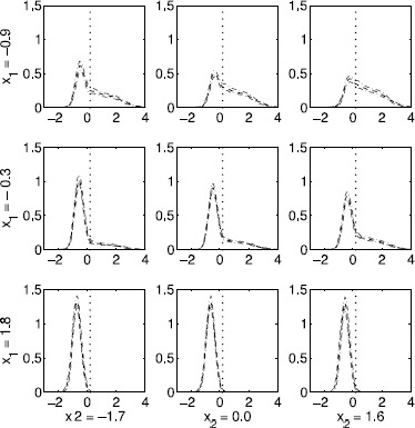
Figure 23.8  Predictive (dashed) conditional response density p(yx) and 95% credible intervals (dash-dotted) with normalized x₁ (insulin sensitivity) and x₂ (age) varying among 5th, 50th, 95th empirical percentiles.

The dependent Dirichlet process (DDP) was originally proposed by MacEachern (1999, 2000) and was subsequently used to develop Anova models of random distributions by De Iorio et al. (2004) and for nonparametric spatial data analysis by Gelfand, Kottas, and MacEachern (2005). There have been numerous applications in different settings, with De la Cruz-Mesia, Quintana, and Muller (2009) using DDPs for semiparametric Bayes classification from longitudinal predictors and Dunson and Peddada (2008) developing an alternative restricted DDP for modeling of stochastically ordered densities. Wang and Dunson (2011b) recently developed restricted DDP mixtures for modeling of densities that are stochastically nondecreasing in a continuous predictor. Most of the focus has been on DDPs with fixed probability weights on the mixture components, but Griffin and Steel (2006) propose an order-based DDP to allow varying weights, and Chung and Dunson (2011) propose a local DP that allows varying weights in a related but simpler manner. Hierarchical DPs (Teh et al., 2006) and nested DPs (Rodriguez, Dunson, and Gelfand, 2009) are applications of the DDP framework to hierarchical dependence structures.

There is a rich literature on alternatives to DDPs for formulating dependence in random probability measures. One key advance was the approach of Muller, Quintana, and Rosner (2004), which formulated dependence in group-specific random probability measures by using convex combinations of a global random probability measure (RPM) with group-specific RPMs. This convex combinations strategy was extended to accommodate continuously varying collections of RPMs by Dunson, Pillai, and Park (2007) using kernel-weighted convex combinations of DPs. An alternative strategy has relied on generalized stick-breaking processes, which replace the beta random variables in the DP stick-breaking representation with more complex forms. For example, Dunson and Park (2009) propose a kernel stick-breaking process, while Reich and Fuentes (2007) apply a related approach to modeling of hurricane winds. Chung and Dunson (2009) and Rodriguez and Dunson (2011) proposed an alternative probit stick-breaking process, while Ren et al. (2011) instead use a logistic stick-breaking process motivated by imaging applications. Dependent stick-breaking processes for time series of random distributions have been considered by Dunson (2006), Rodriguez and ter Horst (2008), and Griffin and Steel (2011), among others.

There is also a literature on alternatives to stick-breaking processes for characterizing dependence in RPMs, with a recent emphasis on normalized random measures with independent increments (James, Lijoi, and Prunster, 2009). For example, Griffin (2011) proposes a class of priors for time-varying random probability measures through normalizing stochastic processes derived from Ornstein-Uhlenbeck processes.

23.8   Exercises

1.  The following exercise is useful to gain familiarity with posterior computation and inferences for the Dirichlet process mixture of Gaussian models:

(a)   Simulate data from the following mixture of normals:

(b)   Use the density() function in R to obtain a non-Bayesian estimate of the density and plot this estimate versus the true density.

(c)   Apply the finite mixture model Gibbs sampler described in Chapter 22 for k = 20, α = α/k, α = 1, μ₀ = 0, and κ= α_τ = b_τ = α = 1.

(d)   Run the blocked Gibbs sampler for N = 20 and the same hyperparameter specification.

(e)   Compare the resulting density estimates.

For sufficiently many MCMC iterations and sufficiently large truncation levels k, N, the density estimates obtained via the finite Dirichlet approximation and truncated stick-breaking approximations to the DPM of Gaussians should be similar.

2.  To get an intuition for the impact of α and P₀, repeat the previous exercise but with:

(a)   A higher value of α, such as α = 10

(b)   A gamma hyperprior distribution on α, with a_α = b_α = 0.1

(c)   Much higher variance in the normal-gamma P₀.

3.  Suppose a study is conducted in which patients’ blood pressure is monitored over time, and patients belong to one of 15 different study centers. Interest focuses on predicting blood pressure from age, smoking, and other variables.

(a)   Describe a parametric hierarchical model for these data.

(b)   Modify this model to allow the distribution of the varying parameters to be unknown to allow uncertainty in variability among patients as well as patients within study centers.

(c)   Outline the steps of a Gibbs sampler for the parametric model and how the steps are modified for the semiparametric model.

4.  Suppose we let y_i ~ P with P ~ DP(αP₀), denoting a Dirichlet process prior on the distribution of the data having concentration parameter α and base distribution P₀.

(a)   Show the form of the posterior distribution of P given y₁, …, y_n in the limiting case in which α → 0.

(b)   Generate and plot multiple realizations from this posterior distribution for the galaxy data.

(c)   Describe an algorithm for obtaining point and interval estimates for the expectation and variance of P based on this posterior.

5.  Suppose we have a high-dimensional regression model with coefficients θ₁, …, θ_p with p very large. We would like to define a prior θ_j ~ P, with P ~ π a random probability measure having prior π chosen so that (i) Pr(θ_j = 0) = π₀ with π₀ ~ Beta(a, b); (ii) Pr(θ_j = θ_j’) = κ for any j ≠ j’; (iii) E_P(θ_j) = 0; and (iv) V_P(θ_j) = 4.

(a)   Describe such a prior and show that it has these properties.

(b)   Outline an MCMC algorithm for posterior computation under this prior assuming θ_j’s are coefficients in a Gaussian linear regression model.

6.  Suppose we have conducted a study comparing case and control groups in a biomarker, with abundant historical data available for control patients. Based on fitting a Gaussian mixture model to the historical database, we obtain dictionary densities f₁, …, f_k, which correspond to normal distributions with different location and scale parameters. To simplify inferences for new studies, we treat these dictionary densities as known but model the weights as unknown and varying between groups.

(a)   Define a simple model and prior specification that accomplishes this for case-control data.

(b)   Using this model as a starting point, define a Bayesian approach for nonparametric testing of equivalence in the biomarker density between the case and control groups.

(c)   Provide details on posterior computation and estimation of the hypothesis probabilities for this approach.

(d)   How can this approach be modified to include covariate adjustment?

7.  Consider the 8 schools example of Section 5.5.

(a)   Modify the normal hierarchical model described earlier to instead place a Dirichlet process prior on the distribution of the school-specific treatment effects. How do the results differ from those for the normal hierarchical model?

(b)   Describe clusters of schools that have identical treatment effects.

(c)   Suppose data were also available on classrooms within schools. How could the model be modified to allow the distribution of treatment effects across classrooms within a school to be unknown?

(d)   Comment on the induced clustering structure of the proposed model in terms of clustering schools and classrooms within and across schools.

(e)   This clustering model does not make much sense in the schools example. Describe a setting where the model could be more appropriate.