Native Graph Processing

We’ve discussed the property graph model several times throughout this book. By now you should be familiar with its notion of nodes connected by way of named and directed relationships, with both the nodes and relationships serving as containers for properties. Although the model itself is reasonably consistent across graph database implementations, there are numerous ways to encode and represent the graph in the database engine’s main memory. Of the many different engine architectures, we say that a graph database has native processing capabilities if it exhibits a property called index-free adjacency.

A database engine that utilizes index-free adjacency is one in which each node maintains direct references to its adjacent nodes. Each node, therefore, acts as a micro-index of other nearby nodes, which is much cheaper than using global indexes. It means that query times are independent of the total size of the graph, and are instead simply proportional to the amount of the graph searched.

A nonnative graph database engine, in contrast, uses (global) indexes to link nodes together, as shown in Figure 6-1. These indexes add a layer of indirection to each traversal, thereby incurring greater computational cost. Proponents for native graph processing argue that index-free adjacency is crucial for fast, efficient graph traversals.

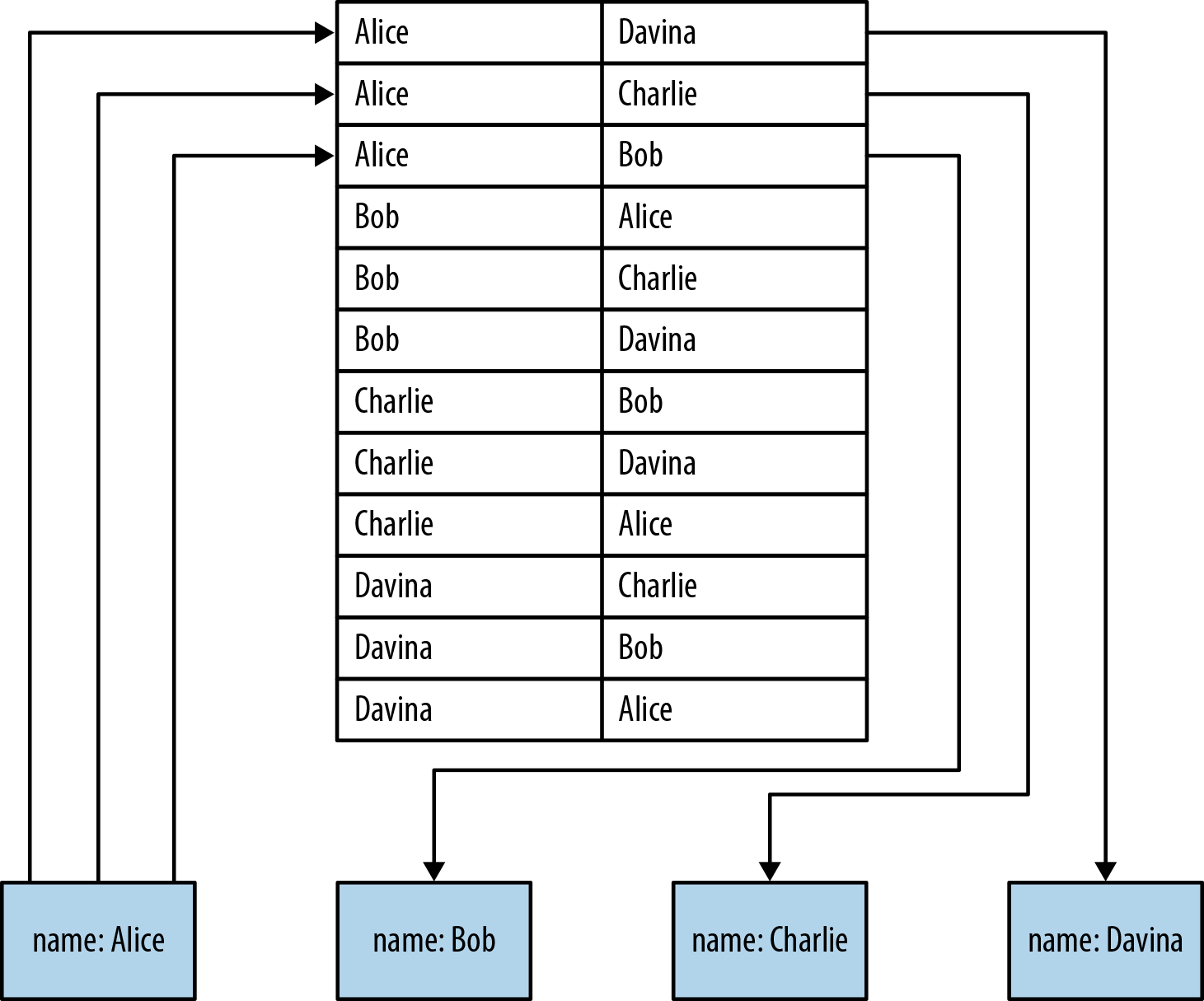
Figure 6-1. Nonnative graph processing engines use indexing to traverse between nodes

Figure 6-1 shows how a nonnative approach to graph processing works. To find Alice’s friends we have first to perform an index lookup, at cost O(log n). This may be acceptable for occasional or shallow lookups, but it quickly becomes expensive when we reverse the direction of the traversal. If, instead of finding Alice’s friends, we wanted to find out who is friends with Alice, we would have to perform multiple index lookups, one for each node that is potentially friends with Alice. This makes the cost far more onerous. Whereas it’s O(log n) cost to find out who are Alice’s friends, it’s O(m log n) to find out who is friends with Alice.

Index lookups can work for small networks, such as the one in Figure 6-1, but are far too costly for queries over larger graphs. Instead of using index lookups to fulfill the role of relationships at query time, graph databases with native graph processing capabilities use index-free adjacency to ensure high-performance traversals. Figure 6-2 shows how relationships eliminate the need for index lookups.

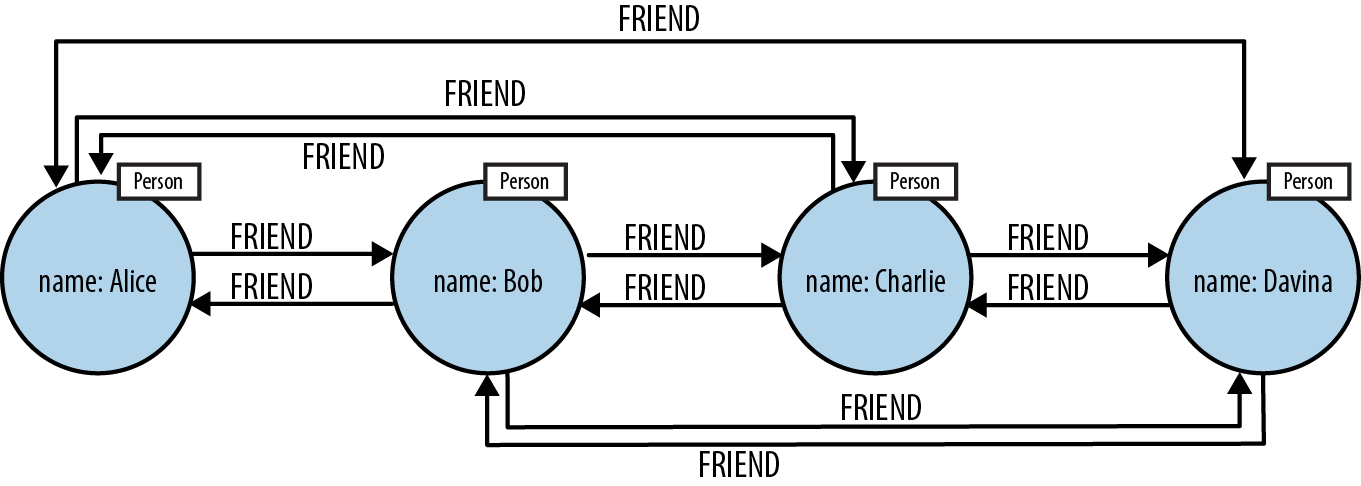
Figure 6-2. Neo4j uses relationships, not indexes, for fast traversals

Recall that in a general-purpose graph database, relationships can be traversed in either direction (tail to head, or head to tail) extremely cheaply. As we see in Figure 6-2, to find Alice’s friends using a graph, we simply follow her outgoing FRIEND relationships, at O(1) cost each. To find who is friends with Alice, we simply follow all of Alice’s incoming FRIEND relationships to their source, again at O(1) cost each.

Given these costs, it’s clear that, in theory at least, graph traversals can be very efficient. But such high-performance traversals only become reality when they are supported by an architecture designed for that purpose.

Native Graph Storage

If index-free adjacency is the key to high-performance traversals, queries, and writes, then one key aspect of the design of a graph database is the way in which graphs are stored. An efficient, native graph storage format supports extremely rapid traversals for arbitrary graph algorithms—an important reason for using graphs. For illustrative purposes we’ll use the Neo4j database as an example of how a graph database is architected.

First, let’s contextualize our discussion by looking at Neo4j’s high-level architecture, presented in Figure 6-3. In what follows we’ll work bottom-up, from the files on disk, through the programmatic APIs, and up to the Cypher query language. Along the way we’ll discuss the performance and dependability characteristics of Neo4j, and the design decisions that make Neo4j a performant, reliable graph database.

Figure 6-3. Neo4j architecture

Neo4j stores graph data in a number of different store files. Each store file contains the data for a specific part of the graph (e.g., there are separate stores for nodes, relationships, labels, and properties). The division of storage responsibilities—particularly the separation of graph structure from property data—facilitates performant graph traversals, even though it means the user’s view of their graph and the actual records on disk are structurally dissimilar. Let’s start our exploration of physical storage by looking at the structure of nodes and relationships on disk as shown in Figure 6-4.¹

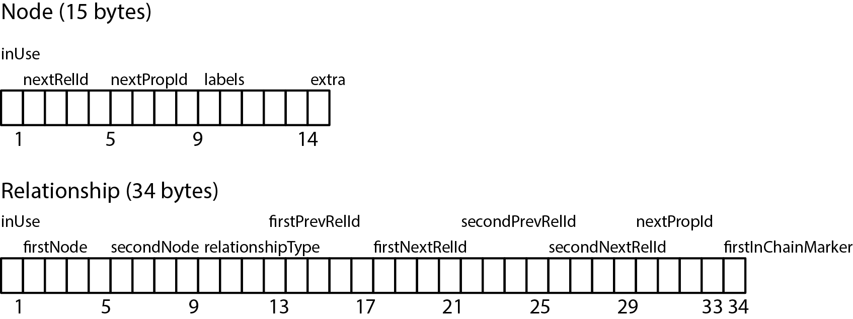
Figure 6-4. Neo4j node and relationship store file record structure

The node store file stores node records. Every node created in the user-level graph ends up in the node store, the physical file for which is neostore.nodestore.db. Like most of the Neo4j store files, the node store is a fixed-size record store, where each record is nine bytes in length. Fixed-size records enable fast lookups for nodes in the store file. If we have a node with id 100, then we know its record begins 900 bytes into the file. Based on this format, the database can directly compute a record’s location, at cost O(1), rather than performing a search, which would be cost O(log n).

The first byte of a node record is the in-use flag. This tells the database whether the record is currently being used to store a node, or whether it can be reclaimed on behalf of a new node (Neo4j’s .id files keep track of unused records). The next four bytes represent the ID of the first relationship connected to the node, and the following four bytes represent the ID of the first property for the node. The five bytes for labels point to the label store for this node (labels can be inlined where there are relatively few of them). The final byte extra is reserved for flags. One such flag is used to identify densely connected nodes, and the rest of the space is reserved for future use. The node record is quite lightweight: it’s really just a handful of pointers to lists of relationships, labels, and properties.

Correspondingly, relationships are stored in the relationship store file, neostore.relationshipstore.db. Like the node store, the relationship store also consists of fixed-sized records. Each relationship record contains the IDs of the nodes at the start and end of the relationship, a pointer to the relationship type (which is stored in the relationship type store), pointers for the next and previous relationship records for each of the start and end nodes, and a flag indicating whether the current record is the first in what’s often called the relationship chain.

In Figure 6-5, we see how the various store files interact on disk. Each of the two node records contains a pointer to that node’s first property and first relationship in a relationship chain. To read a node’s properties, we follow the singly linked list structure beginning with the pointer to the first property. To find a relationship for a node, we follow that node’s relationship pointer to its first relationship (the LIKES relationship in this example). From here, we then follow the doubly linked list of relationships for that particular node (that is, either the start node doubly linked list, or the end node doubly linked list) until we find the relationship we’re interested in. Having found the record for the relationship we want, we can read that relationship’s properties (if there are any) using the same singly linked list structure as is used for node properties, or we can examine the node records for the two nodes the relationship connects using its start node and end node IDs. These IDs, multiplied by the node record size, give the immediate offset of each node in the node store file.

Figure 6-5. How a graph is physically stored in Neo4j

With fixed-sized records and pointer-like record IDs, traversals are implemented simply by chasing pointers around a data structure, which can be performed at very high speed. To traverse a particular relationship from one node to another, the database performs several cheap ID computations (these computations are much cheaper than searching global indexes, as we’d have to do if faking a graph in a nongraph native database):

1. From a given node record, locate the first record in the relationship chain by computing its offset into the relationship store—that is, by multiplying its ID by the fixed relationship record size. This gets us directly to the right record in the relationship store.

2. From the relationship record, look in the second node field to find the ID of the second node. Multiply that ID by the node record size to locate the correct node record in the store.

Should we wish to constrain the traversal to relationships with particular types, we’d add a lookup in the relationship type store. Again, this is a simple multiplication of ID by record size to find the offset for the appropriate relationship type record in the relationship store. Similarly if we choose to constrain by label, we reference the label store.

In addition to the node and relationship stores, which contain the graph structure, we have property store files, which persist the user’s data in key-value pairs. Recall that Neo4j, being a property graph database, allows properties—name-value pairs—to be attached to both nodes and relationships. The property stores, therefore, are referenced from both node and relationship records.

Records in the property store are physically stored in the neostore.propertystore.db file. As with the node and relationship stores, property records are of a fixed size. Each property record consists of four property blocks and the ID of the next property in the property chain (remember, properties are held as a singly linked list on disk as compared to the doubly linked list used in relationship chains). Each property occupies between one and four property blocks—a property record can, therefore, hold a maximum of four properties. A property record holds the property type (Neo4j allows any primitive JVM type, plus strings, plus arrays of the JVM primitive types), and a pointer to the property index file (neostore.propertystore.db.index), which is where the property name is stored. For each property’s value, the record contains either a pointer into a dynamic store record or an inlined value. The dynamic stores allow for storing large property values. There are two dynamic stores: a dynamic string store (neostore.propertystore.db.strings) and a dynamic array store (neostore.propertystore.db.arrays). Dynamic records comprise linked lists of fixed-sized records; a very large string, or large array, may, therefore, occupy more than one dynamic record.

Having an efficient storage layout is only half the picture. Despite the store files having been optimized for rapid traversals, hardware considerations can still have a significant impact on performance. Memory capacity has increased significantly in recent years; nonetheless, very large graphs will still exceed our ability to hold them entirely in main memory. Spinning disks have millisecond seek times in the order of single digits, which, though fast by human standards, are ponderously slow in computing terms. Solid state disks (SSDs) are far better (because there’s no significant seek penalty waiting for platters to rotate), but the path between CPU and disk is still more latent than the path to L2 cache or main memory, which is where ideally we’d like to operate on our graph.

To mitigate the performance characteristics of mechanical/electronic mass storage devices, many graph databases use in-memory caching to provide probabilistic low-latency access to the graph. From Neo4j 2.2, an off-heap cache is used to deliver this performance boost.

As of Neo4j 2.2, Neo4j uses an LRU-K page cache. The page cache is an LRU-K page-affined cache, meaning the cache divides each store into discrete regions, and then holds a fixed number of regions per store file. Pages are evicted from the cache based on a least frequently used (LFU) cache policy, nuanced by page popularity. That is, unpopular pages will be evicted from the cache in preference to popular pages, even if the latter haven’t been touched recently. This policy ensures a statistically optimal use of caching resources.

Programmatic APIs

Although the filesystem and caching infrastructures are fascinating in themselves, developers rarely interact with them directly. Instead, developers manipulate a graph database through a query language, which can be either imperative or declarative. The examples in this book use the Cypher query language, the declarative query language native to Neo4j, because it is an easy language to learn and use. Other APIs exist, however, and depending on what we are doing, we may need to prioritize different concerns. It’s important to understand the choice of APIs and their capabilities when embarking on a new project. If there is any one thing to take away from this section, it is the notion that these APIs can be thought of as a stack, as depicted in Figure 6-6: at the top we prize expressiveness and declarative programming; at the bottom we prize precision, imperative style, and (at the lowest layer) “bare metal” performance.

Figure 6-6. Logical view of the user-facing APIs in Neo4j

We discussed Cypher in some detail in Chapter 3. In the following sections we’ll step through the remaining APIs from the bottom to the top. This API tour is meant to be illustrative. Not all graph databases have the same number of layers, nor necessarily layers that behave and interact in precisely the same way. Each API has its advantages and disadvantages, which you should investigate so you can make an informed decision.

// Index lookup for the node representing the Doctor is omitted for brevity

Iterable<Relationship> relationships =
            doctor.getRelationships( Direction.INCOMING, COMPANION_OF );

for ( Relationship rel : relationships )
{
    Node companionNode = rel.getStartNode();
    if ( companionNode.hasRelationship( Direction.OUTGOING, IS_A ) )
    {
        Relationship singleRelationship = companionNode
                                            .getSingleRelationship( IS_A,
                                                     Direction.OUTGOING );
        Node endNode = singleRelationship.getEndNode();
        if ( endNode.equals( human ) )
        {
            // Found one!
        }
    }
}

Traversal.description()
  .relationships( DoctorWhoRelationships.PLAYED, Direction.INCOMING )
  .breadthFirst()
  .evaluator( new Evaluator()
  {
    public Evaluation evaluate( Path path )
    {
      if ( path.endNode().hasRelationship(
                            DoctorWhoRelationships.REGENERATED_TO ) )
      {
        return Evaluation.INCLUDE_AND_CONTINUE;
      }
      else
      {
        return Evaluation.EXCLUDE_AND_CONTINUE;
      }
    }
  } );

Nonfunctional Characteristics

At this point we’ve understood what it means to construct a native graph database, and have seen how some of these graph-native capabilities are implemented, using Neo4j as our example. But to be considered dependable, any data storage technology must provide some level of guarantee as to the durability and accessibility of the stored data.³

One common measure by which relational databases are traditionally evaluated is the number of transactions per second they can process. In the relational world, it is assumed that these transactions uphold the ACID properties (even in the presence of failures) such that data is consistent and recoverable. For nonstop processing and managing of large volumes, a relational database is expected to scale so that many instances are available to process queries and updates, with the loss of an individual instance not unduly affecting the running of the cluster as a whole.

At a high level at least, much the same applies to graph databases. They need to guarantee consistency, recover gracefully from crashes, and prevent data corruption. Further, they need to scale out to provide high availability, and scale up for performance. In the following sections we’ll explore what each of these requirements means for a graph database architecture. Once again, we’ll expand on certain points by delving into Neo4j’s architecture as a means of providing concrete examples. It should be pointed out that not all graph databases are fully ACID. It is important, therefore, to understand the specifics of the transaction model of your chosen database. Neo4j’s ACID transactionality shows the considerable levels of dependability that can be obtained from a graph database—levels we are accustomed to obtaining from enterprise-class relational database management systems.

Scale

The topic of scale has become more important as data volumes have grown. In fact, the problems of data at scale, which have proven difficult to solve with relational databases, have been a substantial motivation for the NOSQL movement. In some sense, graph databases are no different; after all, they also need to scale to meet the workload demands of modern applications. But scale isn’t a simple value like transactions per second. Rather, it’s an aggregate value that we measure across multiple axes.

For graph databases, we will decompose our broad discussion on scale into three key themes:

1. Capacity (graph size)

2. Latency (response time)

3. Read and write throughput

Capacity

Some graph database vendors have chosen to eschew any upper bounds in graph size in exchange for performance and storage cost. Neo4j has taken a somewhat unique approach historically, having maintained a “sweet spot” that achieves faster performance and lower storage (and consequently diminished memory footprint and IO-ops) by optimizing for graph sizes that lie at or below the 95th percentile of use cases. The reason for the trade-off lies in the use of fixed record sizes and pointers, which (as discussed in “Native Graph Storage”) it uses extensively inside of the store. At the time of writing, the current release of Neo4j can support single graphs having tens of billions of nodes, relationships, and properties. This allows for graphs with a social networking dataset roughly the size of Facebook’s.

Note

The Neo4j team has publicly expressed the intention to support 100B+ nodes/relationships/properties in a single graph as part of its roadmap.

How large must a dataset be to take advantage of all of the benefits a graph database has to offer? The answer is, smaller than you might think. For queries of second or third degree, the performance benefits show with datasets having a few single-digit thousand nodes. The higher the degree of the query, the more extreme the delta. The ease-of-development benefits are of course unrelated to data volume, and available regardless of the database size. The authors have seen meaningful production applications range from as small as a few tens of thousands of nodes, and a few hundred thousand relationships, to billions of nodes and relationships.

Latency

Graph databases don’t suffer the same latency problems as traditional relational databases, where the more data we have in tables—and in indexes—the longer the join operations (this simple fact of life is one of the key reasons that performance tuning is nearly always the very top issue on a relational DBA’s mind). With a graph database, most queries follow a pattern whereby an index is used simply to find a starting node (or nodes). The remainder of the traversal then uses a combination of pointer chasing and pattern matching to search the data store. What this means is that, unlike relational databases, performance does not depend on the total size of the dataset, but only on the data being queried. This leads to performance times that are nearly constant (that is, are related to the size of the result set), even as the size of the dataset grows (though as we discussed in Chapter 3, it’s still sensible to tune the structure of the graph to suit the queries, even if we’re dealing with lower data volumes).

Throughput

We might think a graph database would need to scale in the same way as other databases. But this isn’t the case. When we look at IO-intensive application behaviors, we see that a single complex business operation typically reads and writes a set of related data. In other words, the application performs multiple operations on a logical subgraph within the overall dataset. With a graph database such multiple operations can be rolled up into larger, more cohesive operations. Further, with a graph-native store, executing each operation takes less computational effort than the equivalent relational operation. Graphs scale by doing less work for the same outcome.

For example, imagine a publishing scenario in which we’d like to read the latest piece from an author. In a RDBMS we typically select the author’s works by joining the authors table to a table of publications based on matching author ID, and then ordering the publications by publication date and limiting to the newest handful. Depending on the characteristics of the ordering operation, that might be a O(log(n)) operation, which isn’t so very bad.

However, as shown in Figure 6-7, the equivalent graph operation is O(1), meaning constant performance irrespective of dataset size. With a graph we simply follow the outbound relationship called WROTE from the author to the work at the head of a list (or tree) of published articles. Should we wish to find older publications, we simply follow the PREV relationships and iterate through a linked list (or, alternatively, recurse through a tree). Writes follow suit because we always insert new publications at the head of the list (or root of a tree), which is another constant time operation. This compares favorably to the RDBMS alternative, particularly because it naturally maintains constant time performance for reads.

Of course, the most demanding deployments will overwhelm a single machine’s capacity to run queries, and more specifically its I/O throughput. When that happens, it’s straightforward to build a cluster with Neo4j that scales horizontally for high availability and high read throughput. For typical graph workloads, where reads far outstrip writes, this solution architecture can be ideal.

Figure 6-7. Constant time operations for a publishing system

Should we exceed the capacity of a cluster, we can spread a graph across database instances by building sharding logic into the application. Sharding involves the use of a synthetic identifier to join records across database instances at the application level. How well this will perform depends very much on the shape of the graph. Some graphs lend themselves very well to this. Mozilla, for instance, uses the Neo4j graph database as part of its next-generation cloud browser, Pancake. Rather than having a single large graph, it stores a large number of small independent graphs, each tied to an end user. This makes it very easy to scale.

Of course, not all graphs have such convenient boundaries. If our graph is large enough that it needs to be broken up, but no natural boundaries exist, the approach we use is much the same as what we would use with a NOSQL store like MongoDB: we create synthetic keys, and relate records via the application layer using those keys plus some application-level resolution algorithm. The main difference from the MongoDB approach is that a native graph database will provide you with a performance boost anytime you are doing traversals within a database instance, whereas those parts of the traversal that run between instances will run at roughly the same speed as a MongoDB join. Overall performance should be markedly faster, however.

Summary

In this chapter we’ve shown how property graphs are an excellent choice for pragmatic data modeling. We’ve explored the architecture of a graph database, with particular reference to the architecture of Neo4j, and discussed the nonfunctional characteristics of graph database implementations and what it means for them to be dependable.