Chapter 5

How Accountants Measure Opportunity

The chapters up to this point provide great detail about the decision making process. In particular, we have thus far discussed the theory behind opportunity costs, relevant revenues and costs, demand, and production costs. Up to this point, however, we have only dealt with economic theory. Theoretically speaking, decision makers ideally estimate opportunity costs before making decisions. However, managers in the business world seldom have the luxury of being able to assess true opportunity cost because estimating opportunity costs would require the decision maker to evaluate all possible decisions and determining relevant values for each one. For example, the decision to replace old equipment with new equipment might contain the following possibilities: rebuild or improve existing equipment; purchase new equipment; lease new equipment; or do nothing. Each decision will require a different amount of cash. The differences in cash required can then be used to invest in different projects, pay off debt, hire new employees, or increase inventory or supply reserves. Thus, the process of evaluating all of the possibilities would be extremely c:ostly. As a result, managers often rely upon accounting costs as estimates of opportunity costs in order to save time and money.

Accounting Costs

Accounting costs refer to the amount of cash or other asset that must be sacrificed to obtain some benefit or probable future benefit for a firm. These costs are different from opportunity costs because they are backward looking. That is, accounting costs represent the outcome of previous decisions, whereas opportunity costs represent benefits foregone as the result of future decisions. Accounting costs serve three main purposes. The first purpose is to provide information to external users. This is typically referred to as financial accounting and is governed by Generally Accepted Accounting Principles (GAAP), a set of rules developed by the Financial Accounting Standards Board (FASB). GAAP have evolved to provide information in a manner that best describes the financial events of a company; however, rule makers always face the tradeoff between relevancy and reliability. That is, increasing the level of required reliability may, at the same time, decrease the ability of a company to provide relevant information because accounting data often include estimates. For example, bad debt expense is recorded during the period sales are made even though the company has no way of knowing exactly who will default on their payments. A more reliable way to record bad debt expense would be to wait until the accounts become uncollectable. However, this method would decrease the information’s relevancy because it would likely not be available until sometime after the period in which the sales were made, thereby reducing the usefulness of that period’s accounting information for investor and creditor decision making.

Within financial accounting, accounting costs are used to describe a company’s assets on the balance sheet and expenses on the income statement. The two main principles that exist to guide accounting costs in these areas are the historical cost and the matching principles. The historical cost principle requires accountants to record assets at the original cost. With few exceptions, the cost of the asset remains on the books at the price it was originally purchased.¹ Thus, many companies have land or buildings on their books that have recorded values significantly lower than their fair market value. The matching principle requires the matching of expenses to periods in which the benefits are received. For example, a five-year insurance policy purchased for $5,000 would lead to $1,000 of insurance expense for each of the five years. While this is useful for predicting future cash flows and more clearly reflecting the economic reality to investors and creditors, accrual-based profits and losses are not the same as economic profits and losses. From a decision making view, the timing and amount of cash inflows and outflows is what is important. In the case of the insurance expense, the cash outflow at the beginning of the policy is where the decision maker should focus.

The second purpose accounting costs serve is in tax preparation. Taxes represent a large portion of corporate expenses, potentially eating away almost 40% of a company’s profit. Thus, tax-based accounting is a very relevant topic. However, corporate taxes are governed by the Internal Revenue Service Tax Code, which currently has over 72,000 pages. Thus, a discussion of taxes is beyond the scope of this text. The only point worth mentioning concerning taxes is that noncash expenses, such as accounting depreciation can sometimes have cash effects through their impact on tax liabilities.

The third purpose of accounting costs lies in managerial applications. That is, accounting cost data serves to provide managers information useful for making decisions and seeing that those decisions are carried out. Managers of a firm not only have to make decisions based upon the best information available at a given time, but they must also dictate these decisions to others and must make sure those people actually carry out the manager’s decisions. Making sure those decisions are carried out is usually referred to as the control aspect of managerial accounting. Control in this sense does not refer to the use of force or manipulation, but rather a state of equilibrium where the employee does what the employer wants because it is in the employee’s best interest. An example of this is the firm providing some bonus compensation based upon accounting performance. In this case, employees will try harder to increase performance for the company so that they themselves may earn more money. Although studies show most firms prefer to use accounting information for control purposes, the decision making aspect is also very important, as the decision making step precedes that of the need for control. As such, this chapter will in detail discuss how accounting costs are calculated and how different costing methods can lead to less-than-optimal decisions. In particular, we focus on product costing because it is so important to operations and the accounting methods have a large impact on the costs reported.

Inventory Costs

When a company produces inventory,² accountants assign values to the inventory based upon the costs that were incurred to acquire or produce the inventory, not based on its market value or even its replacement value. If a baker was paid $20 an hour to make a cake that had $3 of ingredients in it and it took him 30 minutes to complete the cake, the accountant would say the cake had a cost of $13 ($20/hr × 0.5 hr + $3). Note that these costs represent the costs of an event that has already taken place. That is, accounting costs are backward looking and as such, are not necessarily good for decision making purposes. As mentioned before, this is because the historical cost principle required by the US GAAP requires assets to remain on the books at the costs initially incurred to obtain them.³ Accounting costs do not disclose the fair value that an item can be sold for, nor do they detail what it would cost to create another item under the present market conditions. Instead, they provide a record of an event that has already taken place. Although accounting costs are backward looking and opportunity costs are always forward looking, production costs are usually consistent over short periods of time. As a result, accounting costs may provide reasonable estimates of the opportunity costs of producing or purchasing the same products in situations when costs do not fluctuate rapidly. Nonetheless, it is always important to be mindful of the differences between accounting and opportunity costs when making decisions.

Let us now consider what is included in the cost of inventory. Accounting rules require any costs necessary to manufacture a unit of inventory to be included in the cost or valuation of inventory. If it cost $20 to produce one desk, then the desk will be included in inventory at $20. To understand this better, however, we must ask what costs are necessary to produce a unit of inventory. Some costs are easier to see than others. In particular, let us return to the doughnut example from Chapter 4. What costs are necessary to produce one doughnut? The easiest cost to see is the cost of the materials that go into the doughnut.

Rather than list the prices for eggs, sugar, milk, flour, and vanilla, let us suppose we have doughnut mix which costs $3 per pound. Additionally, assume one pound of this mix makes 60 doughnuts when water is added. Thus, it is easy to see that the cost of the ingredients for one doughnut is 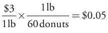. This cost represents the material that is required to make one doughnut and is directly traceable to the doughnut, as demonstrated. Materials that are used in producing inventory are called direct materials. In addition to the materials, an employee must be paid to mix the batter and put it in the oven. Assume the employee is paid $12 an hour and spends six minutes working on one batch of 60 doughnuts. The cost of that employee is also directly traceable to a doughnut through the same method used for the ingredients. Specifically, each doughnut will require of labor. The cost of labor that is used in the manufacturing process is called direct labor because it can be directly traced to the units produced. The cost that is directly attributable to products (direct material and direct labor) together is known as prime cost. Thus, the prime cost of one doughnut is $0.07 in total. Although prime costs are the easiest costs of a unit of inventory to determine, they usually do not represent the entire cost of a unit of inventory.

Are direct labor and direct material the only costs necessary to produce a doughnut? No. Many other costs are needed to produce a doughnut. In addition to direct material and direct labor, manufacturing overhead must also be included into the cost of the inventory. Manufacturing overhead refers to the cost of indirect labor, indirect material, and factory operating costs used for the production of inventory. These costs are called indirect costs because they cannot be directly traced to the inventory produced and they must instead be allocated. Note that the production of doughnuts would not be possible without them, so the company should include them as a cost of production. The cost incurred to convert raw or direct materials into finished inventory (direct labor and manufacturing overhead together) is known as conversion cost.

Indirect costs in the bakery would include the cost of the employee for the time spent cleaning the store or repairing any equipment (indirect labor), the cost of supplies like nonstick solution that is put on baking trays (indirect material), and the cost of electricity, rent, equipment depreciation, and other operating costs (factory operating costs). Assume that these costs amount to $5, on average for every $1 of direct labor cost. In this case, the bakery will allocate $5 of overhead cost to the doughnut for every $1 of direct labor that is traced to the doughnut. Using this ratio, each doughnut should have $0.10 of overhead 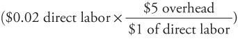allocated to it. The accounting cost to produce one doughnut is $0.17. Remember that only costs necessary for production of inventory are allocated to them. These costs are referred to as product costs and only include direct material, direct labor, and manufacturing overhead. Other costs that are necessary for operations, such as sales or marketing costs, are referred to as period costs and are not allocated to inventory because they are more attributable to the period in question and not necessary for inventory production.

It is important to distinguish between product costs and period costs because, as mentioned before, US GAAP requires expenses to be matched to the period in which the benefits are received. In the case of inventory, the benefit refers to revenues generated by selling a product. Although period costs are expensed in their entirety during the period in which they are incurred, the matching principle dictates that product costs only be recorded as expenses during the periods in which the products actually sell. This expense is called the cost of goods sold expense and it shows up on a company’s income statement. The product costs of goods not yet sold remain on the balance sheet as inventory.

Using Accounting-Derived Costs to Make Decisions

Although allocating overhead costs to inventory is useful for conveying the total cost incurred to manufacture a product, it also diminishes the usefulness of inventory costs for decision making. Specifically, accounting costs are problematic because the allocation process requires making estimates at the beginning of the period and because many of the overhead items allocated to inventory are fixed costs and cannot be avoided. Remember that unavoidable fixed costs, such as rent, should not affect the decision of how many units to produce because those costs will be incurred regardless of what level of production is chosen. Consider the following example:

A frame manufacturer produces picture frames. Their frames require $5 of direct material and $1 of direct labor each. In addition to the prime costs, the company also incurs $8,000 of rent and must allocate it via manufacturing overhead per month. Frankie chooses to allocate this cost to the picture frames via direct labor dollars and, based on his estimated level of total production, requires $2.00 of overhead to be allocated to picture frames for each $1 of direct labor. Table 5.1 exhibits the corresponding price/demand table.

Based on Table 5.1, a rational manager would choose to produce 24 units because that level of production results in a profit of $12,800, which is the highest available possibility. Again, though, it is important to stress that including fixed costs, such as rent, into the decision making process is not a good way to make decisions because fixed costs will not vary with changes in production level. This point is well made by excluding the overhead portion from Table 5.1. Doing so results in Table 5.2.

Based on this table, the company should produce 850 frames and sell them for $23 each. Which table is correct? The overhead (rent, in this case) incurred must be paid for regardless of how the company chooses to prepare its accounting records. Costs that do not vary among choices are not relevant costs and should not be included in the decision making process. Thus, the correct choice is to produce and sell 850 frames for $23 each. Recall from Chapter 3 that demand increases as price decreases. At some point, the additional revenue from selling more units is overcome by the decreases in contribution margin. Due to the overestimation of unit costs, this point is reached more quickly so managers decide to sell fewer units. The result is that fewer units are sold at too high of a price and the company makes $50 less ($14,450 – 14,400). Thus, it should be clear that accounting decisions can have a real impact on firm performance.

Allocating production costs to inventory is required per US GAAP for financial reporting purposes and it is important for properly reflecting economic reality to investors and creditors. Excluding these costs would imply costs of goods sold were lower than they really were and would result in an inflated gross profit. The demonstration above clearly showed how including fixed overhead in the cost of production can potentially lead to less-than optimal decisions being made with respect to price-production schedules. That notwithstanding, the allocation of fixed costs is sometimes used as a control mechanism. Let us consider when it might be desirable to allocate fixed costs.

Taxing Externalities

The benefit of cost allocations is that they affect behavior, allowing firms to curb specific behaviors that results in negative externalities. Externalities are consequences (either benefits or costs) that are experienced by parties not directly related to the decision. For example, acid rain was a negative externality when manufacturers released sulfur dioxide and nitrogen oxides into the atmosphere. The effects of poisoned water sources and eroded structure surfaces were experienced by parties completely unrelated to the release of those pollutants into the air. In contrast, the increase in neighborhood property value that results from a resident landscaping his or her yard is an example of a positive externality. Although the neighbor bore the full cost, the other parties benefited.

The problem with externalities is that the party whose activities generate the externality doesn’t factor them into his decision. For example, a person who decides to get a flu shot weighs the benefit of the shot (reducing the likelihood of contracting the flu) against the costs (the money and time involved in getting the shot). Should he get the shot, other persons also benefit to the extent that they will not contract the flu bug from him. But it is unlikely that the cost/benefit analysis he undertakes includes the benefits to those he comes in contact with.

Negative externalities entail a similar dilemma. In this case, the party’s action imposes an external cost on a third party. Anvil Farms in Boxford, Massachusetts uses bone gel, a byproduct of gelatin made from cattle bones, to fertilize its fields. Unfortunately, the fertilizer emits an odor so noxious that local residents complained to the Board of Health.⁴ Beyond being a nuisance, the odor might conceivably reduce the property value of homes within its range. The problem is that Anvil Farms makes its decision based on its own revenues and costs, not those imposed on neighboring residents.

The economic solution to negative externalities is to force decision makers to incur the costs they would otherwise ignore. London, England initiated congestion pricing in its Central Business District in 2003 to reduce traffic congestion. When driving into the city during peak hours, drivers consider only their own personal costs and benefits. The notion that their decision to drive into the city adds one more car for other drivers to contend with is generally ignored. To force drivers to incur this cost, the city imposed a congestion charge. Cars entering Central London on weekdays between 7 am and 6:30 pm must pay a fee of £8. Video cameras installed throughout the city record license plate numbers and match them against the list of those who paid for the privilege. Violators are fined £40.⁵

The philosophy is that forcing drivers to incur the congestion charge will cause them to consider public transportation as a way to get downtown or to avoid driving into the city during peak hours if it can be avoided. Indeed, after the charge was implemented, traffic decreased by 20%, or 20,000 vehicles/day while bus and subway ridership increased by 14% and 1%, respectively.

Applying the concept to corporations, decisions at the factory level are made by weighing revenues against costs, given that factory supervisors are often rewarded for the profitability of their facility. But production decisions can impose costs on other departments. As long as these costs are borne by outside parties, the plant supervisor has no incentive to consider them. In such circumstances, the supervisor may overproduce the good, increasing the profitability of the plant, but decreasing that of the firm.

A common example with corporations is the allocation of the Human Resources department to departments and then to the products those departments produce. This cost is a relevant production cost because the HR department supports the direct labor force. The cost of the HR department follows a step function as described in Chapter 4. That is, the HR department can only serve a certain number of employees before it must hire additional staff. Between discrete numbers of employees, the HR costs are fixed, and hence, unavoidable. Once the HR department is at maximum capacity and a stairstep point is reached, the additional costs required to hire more employees are avoidable fixed costs.

Just because HR expenses do not rise between stairsteps doesn’t mean there is no negative externality incurred by hiring an additional employee at the plant. Rather, the impact of increasing the number of employees is felt in HR even though its expenses do not rise. That is, the quality of service provided by HR suffers because the additional work must now be covered by the same staff. In fact, it is because the effects are felt that HR decides it needs to add to its personnel. This decrease in quality or higher cost is the externality that companies try to mitigate. Assuming the cost of the HR department represents a significant portion of the overhead, allocating overhead based on some measure of direct labor could be beneficial. By allocating overhead with direct labor hours, management is inclined to use fewer employees. More specifically, allocating the HR department’s cost based on the use of employees actually captures a portion of the opportunity cost of hiring an additional employee. To consider it in another light, imagine the department using employees does not get charged for the HR department. This acts as a discount on the total cost of production, so management from this department would overconsume economic resources through the use of labor. Allocating overhead costs based on a measure of direct labor should result in less direct labor being used. Using less direct labor should result in a lower cost for the Human Resources department. Thus, allocating costs could produce the desired outcome.

Allocating overhead acts as a tax and therefore reduces whatever behavior it is linked to. As pointed out above, this is sometimes useful in approximating the opportunity cost of using a cost driver and reducing the overconsumption of resources. However, the reduction of consumption can sometimes be too large and may result in a much worse overall position than would occur in the absence of cost allocation. The cost of adding one more employee does not increase the costs of the HR department necessarily. After adding enough employees, though, it does become necessary to add another HR representative.

When to Allocate Costs

If possible, it is desirable to allocate costs at their marginal rates, as this method would lead to the most efficient decisions that would be based on real economic costs. Unfortunately, this method is not feasible due to its complexity and the high costs that would have to be incurred to do so. The allocation of costs, instead must rely upon average costs, which are very seldom equal to marginal costs. Thus, the allocation of costs is either done so at a rate that is lower than or higher than marginal costs. When costs are allocated a rate lower than marginal costs, overconsumption is still reduced, just not at the optimal level. A tax that is lower than the marginal rate still decreases consumption of whatever is being taxed, which is beneficial to the company. In contrast, allocating costs when the allocation rate is higher than the marginal rate will result in too much reduction of consumption. This is especially true if external sources of replacement exist. That is, when the allocated rates are higher than marginal costs, managers will reduce consumption by an amount that is larger than desired. This reduction results in the same fixed costs being spread among a smaller allocation base, which leads to an even higher allocation rate. Again, more managers will reduce consumption of the allocation base. This process continues until the rate is so high that no consumption of the allocation base occurs. This phenomenon is known as a death spiral. The takeaway from this is that allocating costs are beneficial from a control standpoint when the allocation rate (average cost) is less than the marginal cost.⁶ Consider the example from a wood company below.

Tables 5.3 and 5.4 illustrate the death spiral. In Table 5.3, the fixed costs are distributed evenly between the three products. Looking only at the profit, the conclusion would be to drop desks from production. Discontinuing desks requires the entire $150,000 of fixed costs to be allocated only to chairs and tables. The profit analysis resulting from this decision is included in Table 5.4. As before, looking at the profit analysis suggests producing tables is unprofitable.

After dropping the tables from production, chairs must absorb the entire $150,000. Producing and selling only chairs will result in a total loss of $70,000 ($200,000 – 120,000 – 150,000). Thus, making decisions based on costs that include fixed portions has led a company from profit to loss. Take note that this example does not imply spreading fixed costs over a larger number of products is what makes the company more profitable. Rather, the company is more profitable when producing both chairs and tables because each has a positive contribution margin.

Turning back to the use of accounting costs for decision-making purposes, let us now consider the specific ways accountants calculate inventory costs and how each of these methods can affect the decision made. The three most common methods used to calculate product costs include the absorption, variable, and activity-based costing (ABC). Of these three methods, absorption costing is the only one that is fully allowed under GAAP. As such, we will first discuss this method for determining the cost of a unit of inventory.

US GAAP requires all costs necessary for the production of a unit of inventory to be included in the cost of that unit of inventory. These costs include those that are easily traceable to inventory, such as direct materials and direct labor. They also include the costs that are more difficult to link to a specific unit of inventory, such as the cost of maintenance, janitorial staff, supervisors, and the human resources and accounting departments.⁷ This second group of costs is referred to as manufacturing overhead and includes all costs necessary for producing inventory that are not direct material or direct labor. These costs include costs for indirect labor, indirect materials, and factory operating costs. As mentioned before, they must be allocated because they cannot be directly traced to each unit produced.

Absorption costing allocates overhead based upon volume of input, not output. That is, the overhead is allocated based upon something that is required to produce overhead rather than dividing overhead by the total number of output. The benefit to using an input rate is it allows companies to allocate overhead during the period via a predetermined overhead rate as opposed to waiting until the end of the period and retrospectively allocating costs. For example, a company has a good idea of what the utility bill will be at the beginning of the month, but they may not actually know what the bill is until the end of the month. Using the actual overhead incurred would require waiting until the end of the period to allocate overhead. Another benefit of using predetermined overhead rates is that costs often fluctuate around some average. These fluctuations are typically small and balance themselves out most of the time so using a predetermined rate provides a consistent cost. A last reason for using units of input rather than output for allocating overhead is that companies produce more than one type of product and these different products require different amounts of prime costs and overhead costs. Using the number of products produced to allocate overhead would certainly undercost a complicated product that takes several steps to produce, while at the same time overcosting products that are simple and quick to make.

Under absorption costing, companies try to choose a unit of input for allocating overhead that is most positively related to the level of overhead. That is, managers of a firm want to as accurately as possible allocate the costs to the units that are producing those costs. If the largest part of overhead comes from machine maintenance or depreciation, then allocating overhead based on machine hours is a logical choice. If the largest portion of overhead comes from having more administration costs to handle all of the direct laborers, then using direct labor hours is probably a good choice. The choice of input is usually limited to machine hours, direct labor hours, direct labor dollars, and direct material dollars. Whichever allocation base a company chooses, it is important to note the allocation of overhead acts as a tax. As described before, the increased cost associated with one more unit of input will make using that unit of input less desirable. To the extent that the input mixes are already at their optimal ratio preallocation, any allocation of costs will shift the input mix away from that point.

For example, a chemical company has several divisions. One of those divisions, Chemicals 1, produces Product X using various chemicals. Chemicals 1 can make Product X using two different solutions that require different amounts of labor to mix. The labor responsible for mixing the units is paid $20 per hour. The production cost schedule is presented in Table 5.5.

According to Table 5.5, Solution A should be used to produce batches of Product X, as it has a lower overall cost by $1,000. If fixed costs are allocated at a rate of $10 per direct labor hour, the new cost schedule is as shown in Table 5.6.

According to the cost schedule in Table 5.6, Solution B should be used because total costs are lower by $3,000. Despite the increased fixed costs allocated due to a higher number of labor hours, the actual fixed cost has not increased. Thus, the result of choosing Solution B will actually still result in a higher cost by $1,000, leading to lower profits for the company as a whole. As this example shows, the allocation of costs can lead to less than optimal results.

Absorption Costing

With all of that said, let us now discuss the process used to actually allocate the overhead. The first step is to estimate the amount of overhead that will be incurred during the period. This process usually involves examining prior period overhead and working with various budgets to determine how much will be consumed during the current period. The next step is to determine which measure of input is most highly correlated with the levels of overhead and choose it as the allocation basis. Finally, estimate the quantity of input that will be used. The predetermined overhead rate, as it is called, is then calculated as

Overhead is then allocated to units during the period as the units of input are used. For example, Foster Glass Company specializes in making glass mugs. At the beginning of 2013, Foster estimates it will have $2,000,000 of fixed manufacturing overhead during the period and chooses to allocate it based upon machine hours. Foster expects to have one million machine hours during the period, which means the predetermined overhead rate will be $2 of overhead for every one machine hour used on a job . On average, it takes 0.05 machine hours to produce a standard glass mug. This translates to $0.10 of overhead allocated to each glass mug ($2 × 0.05).

The amount of overhead applied over a period almost always differs from the actual amount of overhead incurred during a period because the amount of overhead is based on estimates. Consider the following example:

Assume a company manufactures two types of products, the T3 and T4 models. This company estimates it will have $1,400,000 of overhead for the period and will allocate this overhead using direct labor dollars as the allocation base.

Table 5.7 summarizes the estimated production and cost data for the two products. Based on this information, we calculate the predetermined overhead rate as the total estimated overhead divided by the total estimated allocation base, which is of overhead per $1 of direct labor. If the company incurs $250,000 of direct labor expense relating to the production of 5,500 T3s and $490,000 of direct labor expense relating to the production of 10,000 T4s, how much overhead will be allocated during the period?

To determine how much overhead is allocated, we multiply the predetermined overhead rate ($2 overhead per $1 direct labor) by the actual amount of allocation base used ($250,000 for T3 and $490,000 for T4). This calculation indicates $500,000 of overhead will be allocated to T3 units and $980,000 will be allocated to T4 units. The total overhead allocated during the year is $1.48 million. During the period only $1,450,000 was actually spent on overhead. This results in a $30,000 difference between actual and allocated overhead. The difference can be handled in three ways. Most commonly, the difference is adjusted away through the cost of goods sold expense account. In this case, cost of goods sold would be decreased by $30,000 because too much overhead had been allocated to the units, most of which presumably sold. The second way to handle the difference is by reallocating the over/under allocated to the various inventory accounts based on the amount of overhead that is already in the works in process, finished goods, and cost of goods sold accounts.

For example, if the company has ending inventory balances of $29,600, $59,200, and $1,391,200 in its work in process, finished goods, and cost of goods sold accounts respectively, then the treatment of the overallocated overhead would be as shown in Table 5.8.

Notice the account balances are reduced because the actual overhead is less than the company previously assigned during the period. Also, note that the accounts that had the most allocated overhead experiences the highest amount of change. Finally, the last way to account for the difference in allocated and actual overhead is to recompute a retrospective overhead rate based upon actual overhead incurred and the actual allocation base. After calculating the actual overhead rate, use it to apply the accurate amount of overhead to various products during the period. This method is not often used because it is backward looking and requires more work than it is worth. The most common method is to adjust the cost of goods sold account for the difference between allocated and actual overhead.

Although absorption costing is required by US GAAP, it is criticized by many for two main reasons. The first reason is that it creates an incentive to overproduce inventory. Recall that the costs of direct materials, direct labor, variable overhead, and fixed overhead are all included in inventory as product costs. These costs then either go to the income statement through cost of goods sold expense or they remain on the books as ending inventory.

Producing more overhead than can be sold reduces the amount of fixed overhead included in each unit because the fixed cost allocation is done through average costs. The variable costs (direct labor, direct material, and variable overhead) remain relatively constant for each unit produced, but the fixed portion of the product cost decreases with each additional unit produced. By producing more units than can be sold, a portion of the fixed overhead is allocated to the units that remain in ending inventory. Thus, fixed overhead costs that are necessary for producing a normal level of production are hidden in ending inventory, resulting in a lower cost of goods sold and a higher income for the period. Although the cost of goods sold is lower for the period, the fixed costs must still be paid. Thus, the only difference is in how the accounting records report the costs. Additionally, overproduction for the sole purpose of reducing per unit costs presents a case of wasted resources. The variable costs require cash outlays resulting in foregone investments in other projects.

Consider the following cost information for 2013 (Table 5.9):

There is no beginning inventory and the company sells 100,000 units at $5 per unit. The absorption costing method results in a product cost of $1 for each unit ($0.4 + 0.3 + 0.2 + 0.1). In this case, income is 100,000 × $5 per unit minus 100,000 × $1 = $400,000. Notice how they produced 20,000 more units than they sold. This overproduction results in allocating $4,000 of fixed overhead away from the units sold in 2013 to the ending inventory. Again, the fixed overhead costs are still incurred, but the accounting expenses will be deferred until the next period when it will be recognized as the inventory is sold. Several motivations exist for this behavior, but two stand out as most likely. First, most managers receive bonuses based upon some form of accounting earnings. Second, increasing earnings for the period may help the company obtain cheaper debt financing or raise more capital through stock issuances. Thus, managers may very well likely have incentives to overproduce inventory.

Variable Costing

In response to the overproduction problem created by absorption costing, many firms maintain a second set of internal books for calculating period-based income. This method is referred to as variable costing because it only includes variable costs as product costs. Direct materials, direct labor, and variable overhead are all included in product costs, but fixed overhead is treated as a period expense instead. Period expenses are expensed when they are used or expire, in contrast to product expenses, which are only expensed when inventory is sold. This mitigates the incentive for managers to overproduce because the extra units of inventory no longer absorb a portion of the fixed overhead. However, the variable costing method is not allowed for financial reporting purposes because it does not adhere to the matching principal. Maintaining multiple sets of books creates additional expenses for firms and creates the possibility of mistakes. In practice, about 22% of firms use variable costing.⁸ In addition to problems from multiple sets of books, variable costing also introduces the issue of who gets to choose which costs are variable and which costs are fixed. Although this decision is fairly straightforward for most costs like rent and repairs, some costs are more difficult to determine (depreciation, utilities, etc.).

Consider the information from Table 5.9 again. Under the variable costing method, the fixed costs are expensed in whichever period they are produced. Specifically, using variable costing would result in income of 100,000 × $5 per unit minus 100,000 × $0.8 and 120,000 × 0.2 = $396,000. The company produces 120,000 units and only sells 100,000 regardless of which method is chosen. The difference is purely one of accounting. However, the $4,000 of income is still important. Using variable costing provides better data for managers to make pricing decisions. It allows managers to more appropriately assess the profitability of product lines. The number of units produced and sold varies significantly between periods. Variable costing allows managers freedom from biases in costing data based on a predetermined overhead rate that may not be accurate depending on how well estimated allocation base and actual allocation base usage align.

Nonetheless, variable costing still has weaknesses. First, variable costing produces unit costs that are more in line with marginal costs, but still rely upon historical costs. Accounting costs by nature will always represent the outcomes of previous decisions and should be carefully evaluated before being used as a basis for future decisions. Furthermore, variable costing does away with the benefit of allocating fixed costs to proxy for opportunity costs. Assuming a company is in an environment where resources are constrained, the fixed cost allocation can serve a tax to reduce consumption of scarce resources. From a control point of view, there are other ways to reduce managers’ desire to over overproduce inventory. A few examples of alternative techniques include applying a holding charge for inventory based on the firm’s cost of capital, basing managements’ compensation on stock performance if the firm is publicly traded, and stipulating bonuses are only paid when inventory levels are below a certain threshold.

Perhaps a more important concern, as far as decision making goes, is that absorption costing can produce inaccurate product costs. Most companies use a measure of direct labor or direct material to allocate overhead; however, costs can vary with other measures (e.g. machine setups). When firms set machines up for new runs, they often record the labor costs for the setup, but do not note the actual number of setups or what their cause was. Allocating costs based on one measure alone (e.g. direct labor hours) presents a problem because it does not distinguish between products or departments that have low volume and multiple setups or complicated production processes and products or departments with high volume and few setups or simple production processes.

Consider two paint producing plants. The first Plant, Plant W, produces gallons of white paint that comes in different finishes (e.g. flat or satin). This Plant produces 100,000 gallon batches before switching between finishes. The second plant, Plant C, produces white Paint in similar finishes, but also produces the colored paint that is added to white paint in department stores to give the consumer the color he or she wants. Plant C produces 100,000 gallon batches of white paint and 5,000 gallon batches of various colored paints before switching products. Two-thirds of the output from Plant C is white paint with the remainder being colored paint. Plant C has higher overhead costs than Plant W because its employees must spend more time cleaning the vats used to produce paint and setting them up for the different runs. Although most of the output from plant C is white paint, the bulk of the differences between overhead costs in the two plants is due to the smaller batches of colored paint.

Recall, however, that absorption costing allocates overhead based upon a measure of input, such as direct labor or direct material. The result of this allocation method is that white paint in Plant C will capture approximately two-thirds of the overhead. Thus, the cost of white paint from Plant C will be higher than that in Plant W despite the extra costs being the result of the colored paint. An upper level manager considering this data may make two mistakes. The first mistake would be to discontinue the white paint production at Plant C because it can be produced cheaper elsewhere. Notice that this decision would not avoid most of the overhead costs. Instead it would transfer them to the colored paints. The second mistake a manager might make based on this information is to overproduce color paint and sell it at a very low price, failing to recognize the true costs of its production.

Activity-Based Costing

To resolve this issue, some firms have implemented what is called activity-based costing (ABC). In contrast to absorption costing’s use of a single allocation base, ABC assigns indirect costs to separate pools based on what drives their costs and then allocates these costs to products based on the level of activities used in production. Rather than costing activities varying solely with changes in production volume, they are now able to correspond to changes at the unit, batch, product, and facility level. Separating activities into these four levels allows a firm to more accurately assign costs to those products that are driving them.

As the names suggest, unit-level activities are activities, such as assembly processes, that are performed each time one unit of a product is produced. These costs would include utilities associated with the production process (electricity to power the equipment). Batch-level activities include activities that take place each time a new batch is produced and include activities such as machine setups and material handling. Product-level activities are activities that take place in support of particular product lines. Costs that are required for each product line produced include design, modification, creation of instruction manuals, and technical support. Lastly, facility-level activities take place to support the entire facility. This level of activity includes items such as insurance, building depreciation, rent, property taxes, plant maintenance, utility costs incurred not directly related to the production process, and human resources. After tracing costs to the different activities, overhead rates are calculated for each activity and then assigned to the products or jobs based on the amount of activity it takes to produce a unit or to complete the job.

The following provides an example to compare ABC with traditional absorption costing. Suppose a security company produces the following three security systems: simple, advanced, and ultimate. During the year this company produces 60,000 simple, 30,000 advanced, and 10,000 ultimate security systems. The total estimated overhead costs for the period was $8,290,000. This cost consisted of depreciation, research and development, quality assurance, machine setups, and supporting staff salary. Table 5.10 shows the costing information available for the period.

Using this information, we obtain the following application rates by dividing the cost pool by the amount of cost driver, as shown in Table 5.11.

Under ABC, the application rates are then used to allocate the indirect costs to the three specific products. The resulting costs are reported in Table 5.12.

Finally, the cost per unit of each security system is calculated by dividing the total cost for the units by the number of units produced. The results are reported in Table 5.13.

Thus, using ABC results in product costs of $52, 84, and 265 for the simple, advanced, and ultimate security systems respectively. These costs of production are more accurate than if traditional absorption costing had been used because each cost is allocated based on a specific activity that drives the cost.

Using traditional absorption costing and direct labor hours as an allocation base results in an overhead rate of per direct labor hour. Multiplying this rate by the total direct labor hours results in the cost statistics shown in Table 5.14.

Thus, using a traditional absorption-based costing system results in each security system costing $82.90 regardless of whether it is simple, advanced, or ultimate. This simple example is used to illustrate the point that absorption-based costing sometimes results in inaccurate product costs. If the company based its pricing and production decisions upon the absorption-based costs, they would likely try to sell too few simple security systems because its price would be set too high. Not only would this have the result in lower profits initially, but it would ultimately lead to a death spiral because they would produce fewer simple units, thereby increasing the costs of the advanced and ultimate units. Eventually, the company could cease production entirely. Again, this is an extreme example, but the underlying principle holds true.

If ABC is so much better than absorption-based costing and for understanding costs, making decisions, and evaluating performance, then why don’t all firms use it? It seems complexity is a double-edged sword for ABC. The first problem with ABC is that it takes time to set the system up. Someone must go through a company’s production process and determine where all the costs come from and what drives them. This process is both tedious and is partially subjective. That is, department managers may resist allocating costs to activities their departments use considerably. After determining what the costs are and what drives them, additional data on these cost drivers must also be maintained. To capture this data, a firm may have to implement new accounting and information technology systems. Staff will also need to be trained for the new systems. Implementing an ABC system is costly; however, that is not the only issue. Even after establishing an ABC system, the system itself may provide too much information. As more information is produced, the value of each piece of information produced decreases because management may have a difficult time focusing on what is important. Also, the differences between ABC and absorption costing are usually only significant for products that are produced in small quantities at a time. Thus, the benefit for many firms is simply not enough to justify the additional costs incurred to implement and maintain the system. Along this line, research shows that ABC does not have a significant impact on operating performance.⁹ Finally, ABC many times does not adhere to US GAAP because the systems are designed to include nonmanufacturing costs, such as customer support.

When making decisions it is extremely important to be mindful of the fact that accounting costs represent historic costs regardless of the costing method used. Accounting data is important for making decisions because opportunity costs are not usually readily available. However, accounting costs are only useful for making decisions to the extent that they approximate opportunity or marginal costs.

Summary