
Chapter 4
What Your Cost Accountant Can’t Measure: The Economic Theory of Production and Cost
Having determined the relevant revenue associated with a decision, the manager must determine relevant cost. The critical theme of this book is that cost accounting methods rarely report the unit cost figure relevant to the manager’s decision.
We might begin by asking what “unit cost” means. Marketing managers, for example, would be ill-advised to make pricing decisions without knowing what it would cost to produce the output. Although one might ask a cost accountant to define unit cost, it is more telling to pose it to the decision maker. The name “unit cost” implies the cost of making a unit of output. Therefore, if told that unit cost is $15, the individual in charge of pricing would likely conclude that the firm cannot charge a price less than $15 without incurring a loss from the sale of the good.
But this is not necessarily the case. Recall our definition of relevant costs in Chapter 2. Sunk costs refer to expenses that will be incurred regardless of whether the decision is implemented. For that reason, they are never relevant to the decision and should be ignored. In our example, suppose $5 of the $15 unit cost estimate is sunk. If that was the case, any price above $10 would add to the firm’s profits. But how likely is the manager to conclude that he can charge a price as low as $10 without incurring a loss? A more likely scenario is that the manager will incorrectly infer that the entire $15 is relevant, which might cause him to make a pricing error.
Let’s address the definition of unit cost in another example. Suppose the firm has produced three units and is considering a fourth. The manager knows it can sell the unit for $500 and sees that unit cost is equal to $400. Should the firm produce the additional unit? At first glance, the answer appears to be obvious: if the unit cost is $400 and can be sold for $500, it will add $100 to the firm’s profits.
In all likelihood, the unit cost figure reported to the manager is not the cost of producing the fourth unit, but the average cost of producing four units. Suppose, in fact, that the first unit costs $250 to produce, the second costs $350, the third costs $450, and the fourth unit costs $550 to produce. Indeed, the cost of producing four units sums to $1,600, which implies an average of $400/unit. But the unit under consideration costs $550 to produce. If the firm produces the unit and sells it for $500, its profits will fall by $50.
We can relate this latter case to relevant revenue and relevant cost. The unit cost estimate supplied by the cost accountant may be $400, but the relevant cost incurred by producing the fourth unit is $550. This is why selling the fourth unit for $500 causes the firm to incur a loss.
Why didn’t the cost accountant simply report the unit cost to be $550? In all likelihood, the cost accountant does not know the cost of producing each unit individually because it simply cannot be known with certainty. If a firm produces 10,000 units/day, does it know the cost of producing each individual unit? Or is it in a better position to estimate the average cost/unit over a range of 10,000 units, knowing that the cost of each individual unit may vary? “Unit cost” as estimated by cost accounting rarely reports the cost of producing each individual unit, but rather, the average costs incurred over a range of production. But, as our simple example illustrated, the manager who relied on the $400 unit cost estimate to sell the fourth unit for $500 made the wrong decision.
This establishes the focus of this chapter. We will rely on microeconomic principles to derive the economic theory of cost. This will illustrate what the cost accountant would measure in a world of perfect information. In the subsequent chapter, we will review the most commonly used cost accounting methods and how the unit cost estimates may differ from what the manager needs to know. Most importantly, we will be able to see how the imperfections in unit cost estimates can bias the decisions of managers.
Production Theory
Cost theory is derived from the theory of production. To illustrate, assume a worker is paid a wage of $10/hour and the direct materials expense associated with each unit is $5. If the worker is capable of producing one unit per hour, then the unit cost is $15. Suppose the worker is capable of producing two units per hour. In that case, total production costs for the hour are $20 ($10 for direct labor and $10 for direct materials), leading to a unit cost of $10. Note that when the worker became more productive, unit cost decreased. Let’s develop a theory that is sufficiently general as to describe patterns experienced by most firms. Later, we will use the theory to derive a theory of costs.
Mary started a doughnut shop. She rents a space in a small shopping plaza for $1,000/month. She purchased a doughnut fryer for $6,000. A fryer is capable of producing up to 180 doughnuts per hour. For loading and unloading doughnuts, she bought a proofer for $4,000 and $2,000 for a glazing table. Mary spent an additional $15,000 refurbishing the restaurant for sit-down customers.
When the business was just getting started, she hired one worker to make the doughnuts while she operated the cash register. Once the worker learned the ropes, she found he was capable of producing 40 doughnuts per hour. As the popularity of the business grew, Mary found that one worker was insufficient as a bottle-neck of customers appeared at peak morning hours. She hired a second worker to help make the doughnuts. Had the two workers worked individually, and assuming they had equal ability, they could collectively make 80 doughnuts per hour. However, the workers found they could produce more doughnuts by taking on more specialized tasks, thereby divvying up the responsibilities. In doing so, they could produce 100 doughnuts per hour.
As the business grew, Mary needed to add a third worker. As the workers continued to divvy up the responsibilities to maximize production, they found that with three workers, 130 doughnuts could be produced per hour. When three workers proved to be insufficient, she hired a fourth worker. With four workers, an average of 150 doughnuts per hour could be produced. Eventually, Mary settled on five workers, who collectively averaged 160 doughnuts per hour.
Let’s review the pattern between labor hours and production. Total product refers to the total output produced within a given time frame. We begin with the logical assumption that no doughnuts would have been produced without labor. Table 4.1 indicates the total product associated with each quantity of labor hours. As one would expect, doughnut production increases as the number of labor hours rises.1
Table 4.1. Total Product
|
Labor hours |
Total product |
|---|---|
|
0 |
0 |
|
1 |
40 |
|
2 |
100 |
|
3 |
130 |
|
4 |
150 |
|
5 |
160 |
Figure 4.1 graphs the total product curve. Notice that although doughnut production is positively related to the number of labor hours used, it does not follow a linear pattern.
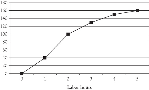
Figure 4.1. Total product.
To understand why total product does not follow a straight line, we will develop another measurement called marginal product. Marginal product refers to the additional output generated by an additional input. Examine the marginal product of each labor hour. The first labor hour results in 40 additional doughnuts. The second labor hour causes doughnut production to rise from 40 to 100, an increase of 60 doughnuts. As noted earlier, had the second worker produced the doughnuts on his own, and assuming he had identical skills to the first worker, doughnut production would have risen by another 40 doughnuts. However, the workers recognized the benefits from specialization; that more doughnuts could be produced each hour by divvying up responsibilities rather than having each person work individually. Economic theory assumes this pattern exists in most production settings: initially, as workers specialize, the marginal product of each additional worker rises.
Note, however, that the pattern of rising marginal product comes to an abrupt halt beginning with the third worker. When the third worker comes aboard, the number of doughnuts produced each hour rises from 100 to 130, or by 30 doughnuts. This is less than the number of doughnuts added by the second worker. Economists refer to this as the law of diminishing marginal returns. The law states that as additional inputs are added to production, eventually each input results in less additional production.
The law has nothing to do with the worker’s ability. In fact, we assume throughout our analysis that the workers are equally skilled. Rather, it’s just a matter of numbers. As an analogy, consider a person who is moving out of an apartment and must carry a sleeper sofa. The sofa is large and awkward, so it would likely take a long time for a single individual to carry it outside to a moving van. If the person had a helper, they would likely grab opposite ends of the sofa and carry it to the van in less than half the time. This is an example of rising marginal product. Suppose a third person helped. Three persons might be able to carry the sofa to the van faster than two persons could, but the third person’s contribution would probably be smaller than that of the second helper. This would constitute an example of diminishing returns.
In the doughnut shop example, although the individuals are trying to work together cohesively, they have to share the workspace and equipment. Production rises with the third worker, but his marginal contribution is smaller than that of either of the first two workers. We can see the diminishing returns with additional workers as well, as the fourth worker adds 20 doughnuts and the fifth worker adds 10. Table 4.2 derives the marginal product associated with each labor hour.
Table 4.2. Marginal Product
|
Labor hours |
Total product |
Marginal product |
|---|---|---|
|
0 |
0 |
– |
|
1 |
40 |
40 |
|
2 |
100 |
60 |
|
3 |
130 |
30 |
|
4 |
150 |
20 |
|
5 |
160 |
10 |
Figure 4.2 plots the marginal product information. The graph clearly indicates that the second worker adds more to total production than the first worker, and that the law of diminishing marginal returns sets in with the third worker.
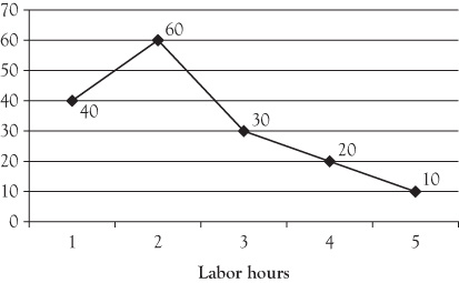
Figure 4.2. Marginal product.
The final measurement of labor productivity is called average product. It measures the average output per input (in this case, the average output per labor hour). Table 4.3 calculates the average product associated with each quantity of labor hours. It is simply the total product divided by the number of labor hours.
Table 4.3. Average Product
|
Labor hours |
Total product |
Marginal product |
Average product |
|---|---|---|---|
|
0 |
0 |
– |
– |
|
1 |
40 |
40 |
40 |
|
2 |
100 |
60 |
50 |
|
3 |
130 |
30 |
43.33 |
|
4 |
150 |
20 |
37.50 |
|
5 |
160 |
10 |
32 |
Note how the average product compares with marginal product for each quantity of labor hours. The two measurements are the same for one labor hour. The first labor hour adds 40 doughnuts to total production, resulting in an average of 40 doughnuts per labor hour.
But note how the two numbers deviate from that point forward. The second labor hour adds 60 doughnuts, causing the average number of doughnuts per labor hour to rise to 50. In general, when the marginal product exceeds the average product, average product will rise. This is analogous to a student’s cumulative GPA and his most recent semester’s GPA. If his cumulative GPA is 3.00 and he earns a 3.25 in his next semester, his cumulative average will rise. In the doughnut example, the average number of doughnuts produced in one labor hour is 40. Because the second labor hour contributes more than 40 doughnuts, the average product will rise (to 50/hour in this example).
Note how the average product declines when the marginal product is below the average. The average number of doughnuts produced over two hours is 50. Because the third labor hour contributes only 30 doughnuts, the average falls to 43.33.
Figure 4.3 shows a generic graph of the marginal and average product curves. The average product has the shape of an inverted U: as the number of labor hours increases, the average number of units produced per labor hour rises, reaches a maximum when the average product is equal to marginal product, and then begins to decline. More specifically, as long as the marginal product exceeds the average product, the average product will continue to rise. As soon as the marginal product is less than the average product, the average product will begin to fall.

Figure 4.3. Graph of a marginal product and average product curve.
Cost Theory
Total Fixed and Total Variable Cost
We will use production theory to derive a theory of costs. Before applying production theory, we need to recall the distinction between fixed costs and variable costs. Fixed costs are expenses that do not vary with output. In the doughnut example, the $1,000 monthly rent is an ongoing fixed cost.2
Variable costs are expenses that vary with production. Wages are a variable cost because the number of doughnuts produced varies with the number of labor hours used. The costs of the ingredients that go into each doughnut (flour, yeast, sugar, etc.) are also variable costs. Suppose each worker is paid $10/hour, including benefits and worker’s compensation. Ingredients expenses average $.12/doughnut. Because our only ongoing fixed cost is paid by the month, we will adapt the hourly production information in Table 4.4 to derive the total variable costs associated with each quantity of doughnuts produced each month (assuming eight hours/day, six days/week, four weeks/month).
Table 4.4. Monthly Total Variable Costs
|
Total product |
Direct labor |
Direct materials |
Total variable cost |
|---|---|---|---|
|
0 |
$0 |
$0 |
$0 |
|
7,680 |
$1,920 |
$922 |
$2,842 |
|
19,200 |
$3,840 |
$2,304 |
$6,144 |
|
24,960 |
$5,760 |
$2,995 |
$8,755 |
|
28,800 |
$7,680 |
$3,456 |
$11,136 |
|
30,720 |
$9,600 |
$3,686 |
$13,286 |
We know that one worker can produce 40 doughnuts per hour. If that individual works eight hours/day, six days/week for four weeks, 7,680 doughnuts will be produced each month. The direct labor cost will be $10/hour × 192 hours, or $1,920. The direct materials cost will be 7,680 doughnuts × $.12/doughnut, or $922. The total variable cost associated with producing 7,680 doughnuts is $2,842. Two workers can produce 100 doughnuts/hour or 19,200/month. Direct labor expenses will equal $10/hour × 192 hours × two workers or $3,840. Direct materials expenses will be equal to $.12/doughnut × 19,200 doughnuts, or $2,304. Thus, the total variable cost of producing 19,200 doughnuts will be $6,144. The remainder of the table shows the costs associated with the doughnuts produced by three, four, and five workers.
A graph of the doughnut shop’s total variable costs appears in Figure 4.4. As the graph illustrates, the firm’s total variable costs rise as the number of doughnuts produced increases.

Figure 4.4. Total variable costs.
If we sum the total fixed and total variable costs together, we get the total cost associated with each quantity of doughnuts. This is shown in Table 4.5. Note that the firm’s total costs begin with the total fixed cost and rise as the quantity of output rises. A graph of the total cost data, combined with the total variable and total fixed cost appears in Figure 4.5.
Table 4.5. Total Fixed, Total Variable, and Total Cost
|
Total product |
Total fixed cost |
Total variable cost |
Total cost |
|---|---|---|---|
|
0 |
$1,000 |
$0 |
$1,000 |
|
7,680 |
$1,000 |
$2,842 |
$3,842 |
|
19,200 |
$1,000 |
$6,144 |
$7,144 |
|
24,960 |
$1,000 |
$8,755 |
$9,755 |
|
28,800 |
$1,000 |
$11,136 |
$12,136 |
|
30,720 |
$1,000 |
$13,286 |
$14,286 |

Figure 4.5. Total fixed, total variable, and total cost curves.
Average Fixed and Variable Cost
Many product-related decisions are based on estimates of unit costs. Let’s take the data for the doughnut shop and convert them into average costs. First, let’s derive the average fixed cost which measures the fixed cost per doughnut. As noted earlier, the shop incurs $1,000 in monthly fixed costs. If we divide $1,000 by the number of doughnuts produced each month, we can determine the average fixed cost. As Table 4.6 indicates, the average fixed cost declines as more doughnuts are produced. This should be fairly intuitive: because total fixed costs do not change with production, the fixed cost per doughnut decreases as more doughnuts are produced. A graph of the average fixed cost data appears in Figure 4.6.
Table 4.6. Average Fixed Cost
|
Total product |
Average fixed cost |
|---|---|
|
0 |
– |
|
7,680 |
$0.130 |
|
19,200 |
$0.052 |
|
24,960 |
$0.040 |
|
28,800 |
$0.035 |
|
30,720 |
$0.033 |

Figure 4.6. Average fixed cost.
The notion that average fixed cost decreases as production increases is not particularly insightful, nor is it very useful for decision making. A more useful measure is the average variable cost, or the variable cost per unit. Because variable costs are incurred each time a unit is produced, it is critical that managers charge a price that will at least cover this cost. Average variable cost is calculated by dividing the total variable cost by the number of units produced. Based on the doughnut data, the average variable cost at each output level appears in Table 4.7.
Table 4.7. Average Variable Cost
|
Total product |
Total variable cost |
Average variable cost |
|---|---|---|
|
0 |
$0 |
– |
|
7,680 |
$2,842 |
$0.37 |
|
19,200 |
$6,144 |
$0.32 |
|
24,960 |
$8,755 |
$0.35 |
|
28,800 |
$11,136 |
$0.39 |
|
30,720 |
$13,286 |
$0.43 |
The graph of the average variable cost data appears in Figure 4.7. Note that the average variable cost is U shaped. As production rises, the variable expense per unit declines at first, but eventually rises. The U shape of average variable cost can be traced to the inverted U shape of average product. We noted that as more labor hours were employed, the average output per labor hour increased, reached a maximum, and then declined. This helps one to see the relationship between average product and average variable cost. If the average output per labor hour rises, the average labor expense per unit necessarily decreases. As an analogy, consider the relationship between gas mileage (a.k.a. the average productivity of your car) and the gasoline cost per mile (a.k.a. average variable cost). As your miles per gallon increases, your gasoline cost per mile decreases, and vice versa. The same is true in production: as average product rises, average variable cost falls. Likewise, as average product declines, average variable costs rise.
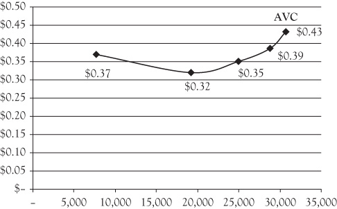
Figure 4.7. Average variable cost.
If we sum the average fixed and average variable costs, we get the average total cost, or the average total expenditure per unit. Table 4.8 shows that as output rises, average total cost decreases. In fact, this is only true up to a point. We know that as output rises, average fixed cost continually decreases while average variable cost falls initially, but eventually rises. But as production continues to rise, average fixed cost becomes negligible.
Table 4.8. Average Variable Cost
|
Total product |
Average fixed cost |
Average variable cost |
Average total cost |
|---|---|---|---|
|
0 |
– |
– |
– |
|
7,680 |
$0.130 |
$0.37 |
$0.50 |
|
19,200 |
$0.052 |
$0.32 |
$0.37 |
|
24,960 |
$0.040 |
$0.35 |
$0.39 |
|
28,800 |
$0.035 |
$0.39 |
$0.42 |
|
30,720 |
$0.033 |
$0.43 |
$0.47 |
Noting that average total cost eventually rises as production increases, Figure 4.8 combines the average fixed and average variable cost curves from Figures 4.6 and 4.7 and adds the average total cost data. Whereas average fixed cost steadily declines with production, average variable cost and average total cost exhibit a U shape.

Figure 4.8. Average fixed cost, average variable cost, and average total cost.
Marginal Cost
The most important measure of unit cost is marginal cost. Marginal cost is the additional cost of producing an additional unit of output. To illustrate its importance, suppose someone approaches a contractor about building a house. He’s selected the house from a book of housing plans and presents it to the contractor. Before they go ahead with the construction, the contractor must provide the individual with a quote. Knowing that the person is likely to solicit quotes from competing contractors, the quote must cover the cost of the construction and offer an acceptable profit. If the contractor quotes too high a price, a competing contractor may undercut him. If the quote is too low, the contractor may lose money on the house.
Marginal cost in this context is the cost of producing this house. It does not serve the interests of the contractor to base his quote on the cost of building the average house, given that this house may be more or less expensive to build than the average house. Likewise, it does not serve the contractor to base his quote on the cost of identical houses in the past if lumber prices have been rising.
Let’s review the data for the doughnut shop and demonstrate why marginal cost is difficult to measure with certainty. Table 4.9 shows the hourly variable costs associated with each quantity of doughnuts. We focus only on variable costs because fixed costs do not vary with the number of doughnuts produced.
Table 4.9. Hourly Doughnut Shop Variable Costs
|
Total product |
Total variable cost |
|---|---|
|
0 |
$0 |
|
40 |
$14.80 |
|
100 |
$32 |
|
130 |
$45.60 |
|
150 |
$58 |
|
160 |
$69.20 |
Examining the table, what is the marginal cost of the 80th doughnut? The table does not show us. We know the cost of making 40 doughnuts and the cost of making 100 doughnuts, but we do not know the cost of making the 80th doughnut. The table only allows us to measure changes in total costs that occur across discrete changes in production. For example, we know that increasing production from zero doughnuts to 40 doughnuts causes expenses to rise by $14.80. We also know that increasing production from 40 doughnuts to 100 doughnuts causes the shop’s operating costs to rise by $17.20.
Although the table does not reveal the marginal cost of the 80th doughnut, let’s manipulate the data to get the best estimate we can. Table 4.10 creates a new column that shows the change in total variable cost divided by the change in production.
Table 4.10. Problems in Estimating Marginal Cost
|
Total product |
Total variable cost |
Change in total variable cost/change in production |
|---|---|---|
|
0 |
$0 |
|
|
40 |
$14.80 |
($14.80 – $0)/40 = $.37 |
|
100 |
$32 |
($32 – $14.80)/60 = $.29 |
|
130 |
$45.60 |
($45.60 – $32)/30 = $.45 |
|
150 |
$58 |
($58 – $45.60)/20 = $.62 |
|
160 |
$69.20 |
($69.20 – $58)/10 = $1.12 |
As the table indicates, the change in total variable cost resulting from a given change in production varies. But let’s go back to our previous question: what is the marginal cost of the 80th doughnut? As the table indicates, we still don’t know. All we really know is that the average cost of producing doughnuts 41 through 100 is $.29. But does that mean that each of those doughnuts cost exactly $.29 to produce?
The table suggests that this is unlikely because the costs differ between production levels. The average cost of the first 40 doughnuts is $.37 and the average cost of doughnuts 101–130 is $.45. If the average cost across production levels differs, it is quite likely that the cost of each unit within a given production level will vary as well.
If we define marginal cost as the cost of producing each individual unit, we can see that Table 4.10 doesn’t really report marginal cost. Instead, the numbers reveal the average variable cost within discrete levels of production. If the average doughnut between 40 and 100 costs $.29 to make, some of those doughnuts have a marginal cost that is less than $.29 and some of them have a marginal cost that is greater than $.29.
This illustrates the problem that cost accountants face when measuring unit cost. It also affects managers who rely on unit cost estimates to make decisions. Most cost accounting methods report unit cost estimates similar to those that appear in Table 4.10. But because the true marginal cost of each unit is unknown, managers rely on the average variable cost measure as the best estimate of the marginal cost of each unit.
Why might this be problematic? Let’s incorporate demand analysis. Suppose 80 doughnuts are demanded at a price of $.40. Should the doughnut shop set its price at $.40 and produce 80 doughnuts? The doughnut shop does not have precise information that allows it to estimate the marginal cost of each individual doughnut. Table 4.10 states that the average cost of producing doughnuts 41–100 is $.29, but we know that each of those doughnuts does not cost exactly $.29 to produce. Given that the average variable cost of doughnuts 101–130 is $.45, the marginal cost of each doughnut must begin to rise somewhere between 41 and 100. Any doughnut that costs more than $.40 to produce will be sold at a loss. But the doughnut shop lacks the necessary data to determine which doughnuts can be sold profitably for $.40 and which cannot.
If we examine Table 4.10, we see that the change in total variable costs divided by the change in output falls initially, but then rises. Let’s combine the numbers in the table with economic theory to explain the likely patterns in marginal cost. Earlier, we noted that average variable cost was the mirror image of average product: if the average output per labor hour was rising, the average labor cost per unit must be falling. The same relationship exists between marginal product and marginal cost. If the marginal productivity of a labor hour rises, the marginal cost of the output produced must decrease. This point was made in the example at the beginning of the chapter. When the marginal product of the worker increased from one unit/hour to two units/hour, the marginal cost of the units decreased from $15 to $10.
Economic theory suggests that marginal product rises initially, but then falls once the law of diminishing returns sets in. If marginal cost follows the inverse pattern of marginal product, the marginal cost of each unit falls initially, but eventually rises. Figure 4.9 shows a graph of the marginal product curve and its corresponding marginal cost curve. As the figure illustrates, marginal cost is at its lowest when marginal product is at its highest. More importantly, the figure shows that for the most part, marginal cost is rising. This implies that once diminishing returns set in, each unit costs more to produce than the previous unit.
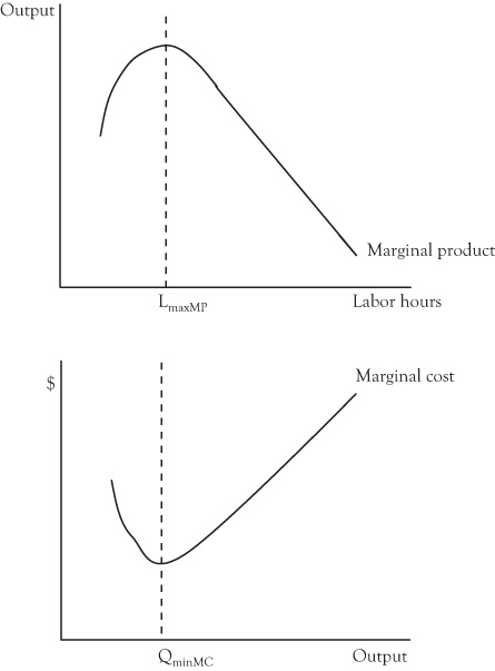
Figure 4.9. Graph of a marginal product and marginal cost curve.
The Profit-Maximizing Price and Output
Let’s incorporate a demand schedule and combine it with the cost data to determine the optimal price and output level. Table 4.11 shows the firm’s demand and cost schedules.
Table 4.11. The Profit-Maximizing Price and Output
|
Price |
Quantity |
Total revenue |
Relevant revenue |
Total variable cost |
Revenue cost |
|---|---|---|---|---|---|
|
|
0 |
$0 |
– |
$0 |
– |
|
$1 |
40 |
$40 |
$40 |
$14.80 |
$14.80 |
|
$.90 |
100 |
$90 |
$50 |
$32 |
$17.20 |
|
$.75 |
130 |
$97.50 |
$7.50 |
$45.60 |
$13.60 |
|
$.60 |
150 |
$90 |
($7.50) |
$58 |
$12.40 |
|
$.40 |
160 |
$64 |
($26) |
$69.20 |
$11.20 |
We can approach the firm’s profit-maximizing price and output using relevant revenue/relevant cost analysis. The first decision Mary must make is whether to produce the first 40 doughnuts (i.e. the production generated by the first worker). The relevant revenue is the amount by which revenue changes if the doughnuts are produced, or $40. The costs will increase by $14.80. Therefore, the profit generated by the doughnut shop each hour will rise by $25.20.
Next, Mary must decide whether to hire another worker to assist the first one. If the second worker is hired, hourly doughnut production will rise from 40 to 100. Because more doughnuts will be produced, the law of demand will require Mary to drop the price from $1 to $.90 to assure they will all be sold. As the table indicates, increasing hourly production from 40 doughnuts to 100 will cause revenues to rise by $50 whereas costs increase by $17.20. Hourly profits will rise by $32.80 if the additional 60 doughnuts per hour are produced.
Should hourly production rise to 130? The law of demand suggests that if hourly production increases to 130, Mary will have to drop the price to $.75. This will cause revenues to increase by $7.50. However, costs will rise by $13.60. If Mary hires the third worker, the shop’s profits will decline by $6.10 per hour. This implies that profits are highest when 100 doughnuts are produced per hour, and priced at $.90/doughnut.
Let’s take the same analysis and look at it from the perspective of changes in revenue per unit and changes in costs per unit. In other words, we are comparing marginal revenue and our best available estimate of marginal cost. Table 4.12 adapts the information in Table 4.11.
Table 4.12. Marginal Revenue/Marginal Cost Analysis
|
Price |
Quantity |
Total revenue |
Marginal revenue (change in TR/ change in Q) |
Total variable cost |
Marginal cost estimate (change in TVC/ change in Q) |
|---|---|---|---|---|---|
|
|
0 |
$0 |
– |
$0 |
– |
|
$1 |
40 |
$40 |
$1 |
$14.80 |
$.37 |
|
$.90 |
100 |
$90 |
$.83 |
$32 |
$.29 |
|
$.75 |
130 |
$97.50 |
$.25 |
$45.60 |
$.45 |
|
$.60 |
150 |
$90 |
($.38) |
$58 |
$.62 |
|
$.40 |
160 |
$64 |
($2.60) |
$69.20 |
$1.12 |
As the table indicates, the first 40 doughnuts will generate an average of $1/doughnut in additional revenues while adding an average of $.37/doughnut to costs. This suggests that the first 40 doughnuts will add to Mary’s profits. The next 60 doughnuts generate an additional $.83/doughnut in revenue, while adding $.29/doughnut to the shop’s costs. On average, these doughnuts will also add to the shop’s profits. Mary should not increase production to 130. If she does, the additional revenue per doughnut ($.25) is less than the added cost ($.45).
But we’ve already noted that the cost figures in Table 4.12 do not accurately report marginal cost. Instead, they report average variable cost between discrete output levels. Even so, the table provides insights that we will use to derive a theory of profit maximization if marginal cost was known. The analysis suggests that each doughnut whose marginal revenue exceeds its marginal cost will add to the shop’s profits. If the marginal cost of the doughnut is greater than its marginal revenue, the doughnut will decrease the firm’s profits. Demand theory suggests that marginal revenue gradually declines as production increases, while marginal cost increases with production after diminishing returns sets in. Therefore, Mary will eventually reach a point that the marginal cost of producing additional doughnuts exceeds the marginal revenue. Increasing production into this range will cause profits to fall.
Figure 4.10 shows the implications of marginal revenue/marginal cost analysis using demand and cost theory. The firm will produce every unit for which the marginal revenue is greater than the marginal cost, but will not produce any unit for which the marginal cost exceeds the marginal revenue. As the figure indicates, the firm will maximize its profits by producing Q* units. Given the law of demand, the highest price that will allow Q* units to be sold is P*. No other price/quantity combination will be more profitable.
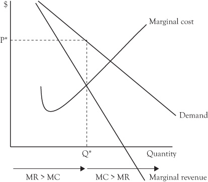
Figure 4.10. Profit-maximizing price and output.
This brings us back to our original point. Figure 4.10 illustrates what the firm wishes to do. Its goal is to determine the price/output level that will maximize profits. In other words, each firm wants to identify P* and Q*. But cost accounting does not report marginal cost. Instead, average variable cost estimates are frequently used as the best available estimate of marginal cost. How might that bias the manager’s pricing/output decision?
Let’s retreat to production theory to determine how marginal cost relates to average variable cost. If marginal cost is inversely related to marginal product, and if average variable cost is inversely related to average product, similar patterns must arise in costs. Specifically, theory states that marginal cost should initially decrease with production. Accordingly, average variable cost should fall because decreasing marginal cost brings the average down. Once diminishing returns sets in, marginal cost will begin to rise. However, as long as marginal cost is less than average variable cost, it will continue to pull the average down. Eventually, marginal cost will exceed average variable cost. Beyond this point, average variable cost will rise. This implies that average variable cost will be at its lowest level when marginal cost is equal to average variable cost. This is shown in Figure 4.11.

Figure 4.11. Marginal cost and average variable cost.
Note how average variable cost and marginal cost are identical at only two output levels (the first unit and QminAVC). If the cost accounting method reports average variable cost as its best available proxy for marginal cost, unit cost will be overestimated for all output levels less than QminAVC. This will cause the firm to underproduce and overprice. Similarly, for output levels exceeding QminAVC, the estimated proxy for marginal cost (average variable cost) will be too low. In this case, the firm will be deluded into producing too many units and underpricing its production.
Let’s add one more piece to the cost puzzle. Some cost accounting methods include fixed overhead in their unit cost estimates. This means that the manager is relying on average total cost as the best estimate of marginal cost. How might this bias the manager’s decisions?
Earlier, we noted that the average total cost is the sum of the average fixed cost and the average variable cost. If we include the average total cost curve in the illustration, we get the cost curves depicted in Figure 4.12.
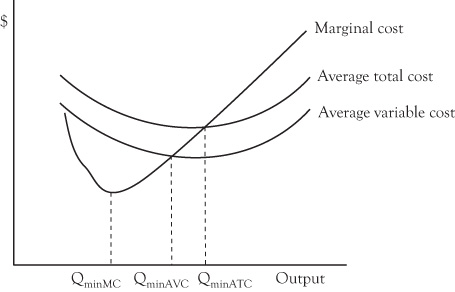
Figure 4.12. Marginal cost, average variable cost, and average total cost.
As Figure 4.12 indicates, the same basic problem exists with average total cost. According to the figure, marginal cost is less than average total cost for all production levels less than QminATC, but exceeds average total cost at output levels greater than QminATC. As with average variable cost, marginal cost is either underestimated or overestimated, leading the manager to either underproduce/overprice or overproduce/underprice.
Step Cost Functions
Earlier, we noted that marginal costs are, by definition, variable costs because fixed costs do not change with production. But if production decisions should be based on marginal costs, and fixed costs are not part of marginal cost, why do some cost accountants use average total cost as their best estimate of marginal cost?
Recall that we can break fixed costs into two categories: unavoidable fixed costs and avoidable fixed costs. Unavoidable fixed costs will not change if the decision is implemented. For this reason, unavoidable fixed costs are sunk costs and not relevant to production decisions. Avoidable fixed costs are fixed costs that will change if a given decision is implemented. This makes them relevant costs.
Let’s use the doughnut shop example to illustrate. The shop paid $1,000/month for rent and purchased a $6,000 fryer capable of making 180 doughnuts per hour. As long as the shop was considering production levels of 180 doughnuts per hour or less, the rent and fryer constitute unavoidable fixed costs because the expenses were unchanged regardless of the output level.
But suppose business had grown to the extent that the shop was capable of selling 250 doughnuts per hour. With only one fryer, it would be incapable of meeting the demand. To meet demand, it would have to purchase a second fryer. Because increasing doughnut production from 180 doughnuts to 250 doughnuts forces the shop to purchase a second fryer, the $6,000 cost of a new fryer is an avoidable fixed cost for any doughnut production exceeding 180/hour. The shop owner would have to determine if the additional doughnut sales justify the additional $6,000 expenditure. If the additional profit contribution is not sufficient to cover the cost of the new fryer, the shop could manage the excess demand by raising the price of the doughnuts.
Let’s bring back some of the data from Table 4.10. The $6,000 cost of the first fryer was not relevant to production or pricing decisions because it was an unavoidable fixed cost. But suppose demand has increased, causing Mary to consider buying a second fryer. This makes the cost of the second fryer an avoidable fixed cost that is relevant to the production decision. Let’s assume the shop is open eight hours/day, 360 days/year. Demand is such that 180 doughnuts per hour (518,400/year) can be sold at a price of $.60, and 250 doughnuts/hour (or 720,000/year) can be sold for $.50. The second fryer reduces some of the logjam that exists with one fryer, increasing the workers’ marginal products. This would cause the variable cost figures to differ from what appeared in Table 4.10. Let’s assume the average variable cost is equal to $.15 at either output level. Can Mary justify buying the second fryer?
Table 4.13 shows the results. As the table indicates, the additional revenue generated as a result of increasing capacity more than covers the relevant costs associated with buying a fryer to increase production.3
Table 4.13. Purchasing a Second Fryer
|
Price |
Quantity |
Total revenue |
Relevant revenue |
Total variable cost + avoidable fixed cost |
Relevant cost |
|---|---|---|---|---|---|
|
$.60 |
518,400 |
$311,040 |
|
$77,760 |
|
|
$.50 |
720,000 |
$360,000 |
$48,960 |
$114,000 |
$36,240 → buy fryer |
Let’s make a slight adjustment to the table. This time, we will assume the price of the doughnuts will have to fall to $.48 if production increases to 250 doughnuts/hour.
Table 4.14 shows the implications. This time, the relevant revenues are not sufficient to cover the relevant cost. Mary should not purchase the second fryer.
Table 4.14. Another Possibility for the Second Fryer
|
Price |
Quantity |
Total revenue |
Relevant revenue |
Total variable cost + avoidable fixed cost |
Relevant cost |
|---|---|---|---|---|---|
|
$.60 |
518,400 |
$311,040 |
|
$77,760 |
|
|
$.48 |
720,000 |
$345,600 |
$34,560 |
$114,000 |
$36,240→ do not buy fryer |
Let’s take the analysis from Tables 4.13 and 4.14 and relate them to cost accounting methods. Earlier, we questioned the logic of using average total cost as the best available proxy for marginal cost. Table 4.14 showed that when the variable costs of increasing doughnut production are combined with the cost of the second fryer, the additional revenues generated by increasing capacity was not sufficient to cover the relevant costs. But the fryer is an example of fixed overhead. If Mary relied only on average variable costs to make her decision (i.e. she ignored the $6,000 cost of the fryer), the relevant cost in Table 4.14 would be shown as $30,240, misleading her into thinking production should be increased to 250 doughnuts/hour.
Does this imply that Mary should rely on average total cost as the most reliable estimate of marginal cost? Not necessarily. Average variable cost was misleading in this example only because Mary was considering an increase in production that necessitated buying a second fryer. For production decisions that can be accommodated with the existing fryer (180 doughnuts/hour or less), the fryer is an unavoidable fixed cost and is not relevant to production decisions.
If we were to plot the fryer expense, we will uncover a step cost function. The expense of a fryer is fixed until it reaches its capacity. Additional doughnut production requires a second fryer. The expenses associated with two fryers remain unchanged until they are both used to capacity. Beyond 360 doughnuts/hour, the fryer expense bumps up to another level. This is shown in Figure 4.13.
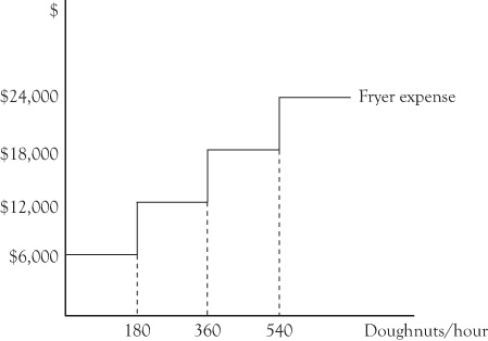
Figure 4.13. Step cost function.
Step cost functions complicate the measurement of unit cost. Within a stairstep, the fryer expense is an unavoidable fixed cost. As we move from one stairstep to another, the expense becomes an avoidable fixed cost. Should unit cost estimates reflect the cost of the fryers? One may take the perspective that because the fryer is not a variable cost, it should not be included in unit cost estimates. However, if production increases entail jumping to another stairstep, the fryer is relevant to production decisions. This suggests that including fixed overhead in the unit cost estimate overstates marginal cost within a stairstep, but is a component of marginal cost across stairsteps.
Let’s complicate matters even further. In our example, the shop knows the precise production levels associated with the stairsteps. If it limits production to 180 doughnuts/hour, it needs one fryer. If it wishes to produce 181–360 doughnuts/hour, it needs two fryers. With many firms, the production levels associated with each stairstep are not known with certainty. Consider a university. The larger the student enrollment, the more faculty members are needed. An additional student does not necessitate an additional faculty member: expanding the class size from 50 students to 51 does not imply a need for more faculty. As enrollments rise, the university may add sections without adding faculty. But eventually, university enrollment approaches a stairstep that requires additional faculty. The precise enrollment level associated with each stairstep is unknown; the university only has a general awareness of the ranges of enrollment that might require additional faculty.
Long-Run Costs
The discussion of step cost functions segues into the economic theory of short-run and long-run costs. In some business disciplines, “short run” is explicitly defined, usually as six months or a year. The economic definition of the short run is much more flexible: we define it as the period of time in which there is at least one fixed cost. No fixed cost is indefinite. Mary signed a lease with high hopes of a profitable venture. But suppose the level of demand was less than anticipated. The monthly rent is an unavoidable fixed cost, but leases expire. Suppose Mary borrowed the funds to buy the fryer and makes monthly payments. If Mary decides to discontinue the business, she will still be obliged to make payments, but eventually the fryer will be paid off. Perhaps she can sell the fryer at some salvage value.
At the other extreme, the business may be so successful that Mary considers opening a second doughnut shop. Or a third. Over the long run, all expenses are either variable or avoidable fixed costs. Economists are reluctant to assign a fixed time frame to what constitutes the “short run” because it will vary by situation. Suppose Mary bought the equipment with cash and signed a year’s lease. In that circumstance, one might reasonably conclude the short run is a year. Had she signed a three-year lease, the short run might be defined as three years.
Are long-run costs simply the summation of short-run costs? For example, can Mary assume that the cost of operating three identical shops simply three times the cost of operating one shop?
Theory suggests that this will not be the case in most circumstances. Recall that the law of diminishing returns causes marginal product to fall as inputs are added to production. Increasing the scale of operations may forestall the onset of diminishing returns. For example, as opposed to buying a second fryer, Mary may have considered buying a larger fryer when the shop was first opened. The incremental cost of a large initial fryer may be less than the cost of a second smaller fryer. If so, the average cost of producing 250 doughnuts per hour may be less than the average cost of producing 180 doughnuts/hour. When increases in production lead to decreases in long run average costs, the firm is experiencing economies of scale.
Increasing production does not always lead to economies of scale. Beyond a given point, large-scale production may lead to additional layers of personnel whose efforts may be difficult to coordinate. This may cause long run average costs to rise with production, resulting in diseconomies of scale.
Economists generally assume that as firms expand their operations over the long run, they experience economies of scale followed by diseconomies of scale. The doughnut shop owner may, for example, find that the average cost associated with two shops is lower than that of one shop, but that the average cost of three shops is higher than that of two shops. This is depicted in Figure 4.14. As the graph shows, the long-run average cost is minimized by operating at Q2, which corresponds to two doughnut shops. As with any decision, the net benefits or cost of expansion should be determined by identifying its relevant revenues and costs.
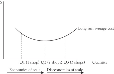
Figure 4.14. Long-run average cost curve.
Summary
•Economic theory predicts that as inputs are initially added to production, marginal product will rise as the inputs become more specialized. Once the law of diminishing returns sets in, the marginal product of each additional input will fall.
•As long as the marginal product of the additional input exceeds the average product, average product will rise. Once marginal product falls below average product, average product will fall. This means that the average product will rise to a maximum level, but will eventually begin to fall.
•Fixed costs refer to costs that do not vary with production. The average fixed cost will fall as more units are produced. Variable costs are expenses that vary with production. Whereas total variable costs will rise as output increases, average variable cost will initially fall as production increases, but will eventually rise. Total costs begin with the firm’s fixed costs and rise as production increases. Average total costs decrease with production initially, but eventually rise.
•Marginal cost is the additional cost generated by an additional unit of output. It falls as marginal product rises, but increases once the law of diminishing returns causes marginal product to fall.
•The firm will maximize profits by producing every unit for which the marginal revenue is greater than the marginal cost. It will lose money on every unit whose marginal cost exceeds its marginal revenue.
•Few firms know the marginal cost of each unit of output. If its cost accounting uses average variable cost as a proxy for marginal cost, the firm may produce too little or too much output. If the firm uses average total cost as a proxy for marginal cost, it will allow fixed costs to influence its production level even though fixed costs are not usually relevant to production decisions.
•Some fixed costs follow step functions. Between discrete ranges of output, these constitute unavoidable fixed costs. At the stairstep, they become avoidable fixed costs. In many instances, the firm does not know with certainty the production level that will necessitate an increase in fixed costs.
•When firms have sufficient time to make changes to overall capacity, theory predicts that firms should initially encounter economies of scale in response to increases in production. This causes average cost to fall. As production continues to rise, the firm eventually faces diseconomies of scale, which causes average costs to rise.