
Chapter 3
Determining Relevant Revenues: Understanding the Buyer
The Law of Demand
1. Individual Demand
The previous chapter was devoted to a discussion of relevant revenues and costs. To maximize profits, firms must determine the changes in revenues (relevant revenues) associated with a given decision. Consumer choice theory can be very useful in helping managers to determine relevant revenues.
To understand consumer behavior, we have to recognize the role of opportunity cost. Consumers don’t have to buy from your firm. From their point of view, the price of your good represents opportunity cost: if they pay $100 to buy your good, they cannot spend it on other goods and services they may value. Thus, the consumer will weigh your good against those produced by competing firms. Even if no viable competitors exist for your product, the consumer may choose to dedicate the $100 to unrelated goods the individual values.
Consumer choice theory allows us to understand how buyers make choices in the face of opportunity cost. Suppose you are going to the ballgame and expect to buy concessions while you’re there. At a break in the game, you decide to buy a beer. A 16-ounce beer costs $5. Five dollars certainly won’t break you, and in fact, you have $20 in your wallet. To you, the issue is not whether you like or could afford a beer, but whether the beer gives you as much satisfaction as anything else you could buy with $5. Hence, you weigh the satisfaction from drinking a beer against the satisfaction you could obtain from spending the $5 on other goods and services. Your decision may or may not hinge on the price of other concessions. You could decide not to buy any concessions at the game and to spend your money after the game on whatever you choose. You may not even spend the money the same day. The key is that you evaluate buying the beer against all other alternatives.
This is the essence of consumer choice theory: to derive a theory that describes a consumer’s behavior. Let’s continue with our ballgame example. You visit the concessions stand. You must decide between buying a hot dog and buying a beer. Suppose hot dogs also cost $5. Because both goods have the same price, you will purchase the good that gives you the most satisfaction. Economists use the word utility to refer to satisfaction. Marginal utility refers to the satisfaction the individual obtains from one more unit of the good. If you decide to buy the hot dog, we can infer that the marginal utility of the first hot dog (MUHD1) gives you more satisfaction than the first beer (MUB1). Later in the game, you return to the concessions stand. This time, you buy the beer. It must be true that the marginal utility from the first beer (MUB1) (i.e. additional satisfaction) exceeds the marginal utility from the second hot dog (MUHD2).
Your buying habits establish the framework that describes consumer demand. You preferred the first hot dog to the first beer, but you would rather have your first beer than your second hot dog. Let’s review your preferences:
1.MUHD1 > MUB1 (the first hot dog is preferred to the first beer)
2.MUB1 > MUHD2 (the first beer is preferred to the second hot dog)If the first hot dog is preferred to the first beer, but the first beer is preferred to the second hot dog, it also follows that the first hot dog is preferred to the second hot dog, or:
3.MUHD1 > MUHD2 (the first hot dog is preferred to the second hot dog)
Economists refer to this as the law of diminishing marginal utility. It suggests that the additional satisfaction derived from each additional unit diminishes as more units are consumed. If this were not true, you would go to the game and spend all of your money on hot dogs. Because consumers spread their money around to buy a wide array of products, we can infer the law of diminishing marginal utility plays a role in virtually all purchase decisions.
If the law of diminishing marginal utility states that each unit provides the buyer with less additional satisfaction, it must also be true that the buyer is willing to spend less on each additional unit. Thus, if the buyer is willing to spend up to $3.75 for the first hot dog, he will be willing to spend less than $3.75 for the second hot dog, and even less for the third hot dog. Suppose the consumer is willing to spend up to $2.50 for the second hot dog, and $1.25 for the third hot dog. This allows us to derive the law of demand. If the price of hot dogs is $3.75, the buyer would only be willing to buy one because the other hot dogs do not provide sufficient satisfaction to justify the opportunity cost. If the price of hot dogs fell to $2.50, he would be willing to buy two hot dogs. The second hot dog now justifies the expenditure, but the third one does not. The law of demand states that as the price of a good rises, the quantity demanded decreases, and vice versa.
The individual’s demand for hot dogs appears in Table 3.1 and is expressed graphically in Figure 3.1.
Table 3.1. Individual Demand Schedule
|
Quantity |
Willing to spend |
|---|---|
|
1 |
$3.75 |
|
2 |
$2.50 |
|
3 |
$1.25 |

Figure 3.1. Individual demand curve.
2. Demand Faced by the Firm
The demand for the good produced by the firm indicates the quantities of a firm’s good or services that buyers are willing and able to buy at each price. It is simply the sum of the quantities demanded by each individual consumer. An example appears in Table 3.2, with the corresponding firm demand curve illustrated in Figure 3.2.
Table 3.2. Demand Schedule for the Firm
|
Price |
Quantity demanded by |
|||
|---|---|---|---|---|
|
Amber |
Bruce |
Casey |
Total demand |
|
|
$3.75 |
0 |
1 |
1 |
2 |
|
$2.50 |
1 |
2 |
1 |
4 |
|
$1.25 |
2 |
2 |
2 |
6 |

Figure 3.2. Firm demand curve.
The Law of Demand and Marginal Revenue
The law of demand asserts that as the price of the good rises, the quantity demanded by consumers falls. Conversely, the law also states that the more units the firm wishes to sell, the lower the price it must charge.
Netflix encountered the law of demand when it developed Qwikster. Netflix established its position in the DVD rental market with its rent-by-mail system. As downloading became increasingly popular, the firm sought to segment its market. Subscribers could continue to order DVDs by mail. Others could subscribe to its cheaper downloading service, which it named Qwikster. But Netflix subscribers could already download in addition to order by mail, so what Netflix saw as a means to segment its market, its subscribers saw as a 60% increase in the price of subscriptions. In response to falling subscriptions and widespread subscriber outrage, Qwikster was abandoned.1
An important component to determining relevant revenue is marginal revenue. Marginal revenue is the additional revenue generated by an additional unit of output. Clearly, when determining whether to increase production, the firm wants to know how much additional revenue will be generated. Such decisions cannot be made in a vacuum. The firm cannot assume that any and all of its additional production can be sold at the existing price. Instead, the quantity it sells is going to be influenced by the law of demand.
At first glance, one might assume that the marginal revenue generated by a unit of output is equal to its price. But this is not the case. To illustrate, examine the information in Table 3.2. If the firm charges $2.50, it can sell four hot dogs. If it lowers the price to $1.25, it can sell six hot dogs. Is the marginal revenue from the two additional hot dogs $2.50 ($1.25 x two additional hot dogs)?
Let’s examine this decision closely. According to Table 3.2, it can sell four hot dogs at a price of $2.50. This would generate revenues totaling $10. If it lowers the price to $1.25, the firm could sell six hot dogs. Note that the firm’s revenue under this price would fall to $7.50. Thus, increasing unit sales from four hot dogs to six hot dogs didn’t cause the firm’s revenue to rise by $2.50; in fact, it caused revenue to fall by $2.50. Why?
If we break the decision down into two parts, we can see what happened. On the one hand, the firm sold two additional hot dogs at a price of $1.25 each. Economists refer to the $2.50 generated by the two hot dogs as the output effect. But this is only half the story. When the firm decided to sell six hot dogs, it lowered the price from $2.50 to $1.25 on all six hot dogs, not just the last two. Therefore, in addition to selling two additional hot dogs for $1.25 each, the firm lowered the price on the first four hot dogs from $2.50 to $1.25. In other words, the firm has to forego $5 ($1.25 on each of the first four hot dogs) in order to sell six hot dogs. The $1.25 price reduction on the first four hot dogs is called the price effect. The marginal revenue is the sum of the output and price effects. In this case, by increasing unit sales from four hot dogs to six hot dogs, the firm’s revenue changed by the sum of the output ($2.50) and price effects (–$5), or a decrease of $2.50.
To develop the relationship between firm demand and marginal revenue, examine Table 3.3. If the firm wishes to sell one unit, it can charge a price as high as $10, which yields $10 in total revenue. The marginal revenue from the first unit, therefore, is $10. If the firm wants to sell two units, it must drop the price from $10 to $9. This will cause revenues to rise from $10 to $18, an increase of $8. If the firm wants to sell three units, it must lower its price from $9 to $8. This will cause revenues to increase by $6 (from $18 to $24).
Table 3.3. Firm Demand and Marginal Revenue
|
Price |
Firm demand |
Total revenue |
Marginal revenue |
|---|---|---|---|
|
$10 |
1 |
$10 |
$10 |
|
$9 |
2 |
$18 |
$8 |
|
$8 |
3 |
$24 |
$6 |
Note that aside from the first unit, the marginal revenue from each unit is less than the price. For example, the second unit can be sold for $9, but it only increases revenues by $8. The third unit can be sold for $8, but it will only cause revenues to rise by $6. Marginal revenue is less than the price because of the price effect; the extra revenue generated by the additional unit is at least partially offset by the lower price on the other units. This can be seen in Figure 3.3. Because marginal revenue is less than the price for all but the first unit, the marginal revenue curve lies below the demand curve.

Figure 3.3. Demand curve and marginal revenue.
The implications of the law of demand on marginal revenue cannot be understated. Sound decision making requires the manager to determine the relevant revenue pertaining to a decision. It is too convenient to assume that marginal revenue consists only of output effects. But the law of demand states that most production increases necessitate lowering the price. For this reason, it is imperative that firms consider potential price effects when determining relevant revenues.
Factors That Change Demand
In addition to price changes, consumers respond to changes in other factors. Suppose the price charged by a competitor rises. As a result, some of his customers may decide to buy from your firm instead, even though you have not changed your price. This is illustrated in Figure 3.4. The original demand curve is shown as D1. At the current price of $10, 100 units are sold. After the competitor increased its price, the demand for your good increased to D2, a shift to the right. This allows you to sell 150 units at the same price. In essence, an increase in the price of a substitute caused the demand for your good to increase.

Figure 3.4. Increase in demand.
Demand can also change if the price of a complementary good changes. An example appears in Figure 3.5. Assume the price of a bag of French fries is $1 and the price of a hamburger is $1.50. At these prices, the demand for fries is characterized by D1, and the quantity of fries demanded is 100. If the price of hamburgers rises to $2, not only will consumers buy fewer hamburgers, they will also purchase fewer bags of fries. Thus, the demand for fries decreases, shifting the demand curve to the left. At the new level of demand, 50 bags of fries are demanded.
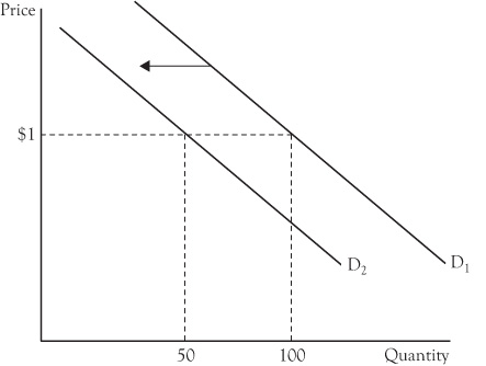
Figure 3.5. Decrease in demand for French fries.
Income changes can also affect demand. Although we generally think that increases in income will increase demand, this is not always the case. When consumer incomes rise, the demand for used cars may fall as consumers substitute into buying new cars. Economists label goods whose demand rises when incomes rise as normal goods. If demand decreases in response to an increase in income (such as our used car example), the good is called an inferior good.
Changes in consumer tastes can cause demand to increase or decrease. Some goods are seasonal in nature. The demand for snow skis rises in the winter and falls in the summer. Some goods become obsolete. As cell phones became more popular, the demand for landline phones decreased.
Changes in price expectations can affect demand. After the terrorist attacks on 9/11, consumers feared gas prices would skyrocket and rushed off to fill their tanks. The result was long gas lines and, ironically, higher gas prices.2 The higher prices were not created by the attacks, but rather, by the panic that led everyone to try to fill their tanks on the same day.
The Price Elasticity of Demand
Another key element of demand theory that is critical to determining relevant revenue is the price elasticity of demand. The law of demand asserts that as the price rises, the quantity demanded falls. The price elasticity of demand expands on the law of demand: it measures the responsiveness of the quantity demanded to price changes. Drivers inevitably grumble about rising gasoline prices. Many individuals regard driving as a necessity because they simply live too far from work, school, or other destinations to walk or ride a bike. Moreover, their cars only run on gas: they can’t pump water into their tanks if the price of gas becomes too costly. As a result, when gas prices rise, consumers may cut back on their gasoline consumption a little, but not by a whole lot. But consumers are less likely to complain about the rising price of frozen yogurt. Unlike gas, frozen yogurt is unlikely to be viewed as a necessity. If the consumer thinks the price is too high, he can simply do without. Moreover, ice cream and frozen custard are reasonably close substitutes for frozen yogurt. If the price of frozen yogurt rises, the consumer can substitute into ice cream.
Let’s illustrate the concept of price elasticity graphically. Figure 3.6 shows the demand curves for gasoline and frozen yogurt. Note that whereas the law of demand holds in both cases, a given increase in the price leads to a larger decrease in the quantity of frozen yogurt demanded relative to the decline in the quantity of gasoline demanded. When the quantity demanded of a given product is relatively responsive to price changes (i.e. frozen yogurt), we say that good has a relatively elastic demand. When the quantity demanded of a good is not very responsive to price changes (i.e. gasoline), we say the good has a relatively inelastic demand.

Figure 3.6. Graphical representation of price elasticity.
What determines price elasticity? We have already covered two determinants. The first is whether the good is a luxury or a necessity. If a good is considered to be a luxury, the prospective buyer may choose not to buy it if the price is too high. This is why the travel industry often suffers during recessions. Families are less likely to go on a vacation if one or more of the parents are unemployed or fears losing his job. If the product is viewed as a necessity, on the other hand, the consumer may have no choice but to continue to buy the good.
Another determinant is the availability of substitutes. When the price of a good rises, they look for cheaper substitutes. When the price of frozen yogurt rises, they can substitute into ice cream, whereas the drivers cannot opt for cheaper substitutes when the price of gasoline rises.
This is why gasoline is a frequent government target for taxation. In 1980, the federal gasoline tax was 4 cents per gallon. By 1993, the tax had risen to its current level of 18.4 cents per gallon. And this is only the federal tax. Each state has its own tax, ranging from roughly ten cents per gallon to 40 cents per gallon.3 Gasoline is a target for taxation because consumers cannot cut back significantly on their gasoline consumption when prices rise.
Another determinant of price elasticity that relates to the availability of substitutes is the definition of the market. Whereas consumers may view the demand for gasoline to be relatively inelastic, the same cannot be said for the gasoline sold at the gas station on the corner of First and Main. Consumers may have few alternatives when the price of gasoline rises, but they can easily substitute away from the gasoline sold at a specific station by purchasing gas from a competing station. Thus, whereas the demand for gasoline may be inelastic, the demand for gas sold by a specific retailer is highly elastic.
Another determinant of price elasticity is the price of the good as a percentage of the consumer’s budget. The National Association for Convenience Stores reported an average gross margin of nearly 47% on warehouse-delivered snack foods at convenience stores in 2008.4 This should not come as a surprise to consumers. A candy bar that might cost $.50 at a supermarket may cost $.75 (50% more) at a convenience store. Why? Undoubtedly, consumers do not make the trip to the convenience store to buy snack foods. In most cases, they enter the store to finalize a gasoline purchase. In deciding whether to buy the candy bar, the consumer is well aware that a better price can be had at a supermarket. But even if the candy bar is cheaper at the supermarket, the opportunity cost of buying it at the convenience store is fairly low, particularly when one considers the time involved in finding a better price. Therefore, we would expect consumers to be relatively price inelastic when it comes to goods that are relatively inexpensive.
Although consumers may claim that they’re willing to pay the additional 50% for convenience, the rationale doesn’t really hold up to scrutiny. Suppose a “convenient” auto dealer was selling a new car for $30,000 whereas a competing dealer on the other side of town was offering the identical car for $20,000. Would the consumer be willing to pay the additional 50% for the convenience? Clearly, the difference between paying 50% more for a candy bar as compared to 50% more for a new car is the opportunity cost of the purchase. Regardless of whether the consumer buys the car at the convenient dealership or the one across town, the opportunity cost of the purchase is sizable. Consequently, the higher the price as a percentage of the consumer’s budget, the more price sensitive the consumer.
Orbitz discovered differences in the willingness to pay for hotels between Mac and PC users. Its own research showed that Mac users are willing to spend as much as 30% more on hotel rooms. Why? According to Forrester Research, the average income for Mac users is $98,560, as compared with an average income of $74,452 for PC users. The knowledge that Mac users were less price sensitive than PC users led Orbitz to steer potential customers who accessed the website on a Mac into pricier hotel rooms.
The final determinant of price elasticity is the time the consumer has to make a purchase. Consider an extreme case. The National Weather Service reports that a hurricane is imminent. When that occurs, coastal residents are in a rush to buy plywood shutters, install them quickly, and drive inland before the storm makes landfall. Under less trying circumstances, these same consumers would shop around for an acceptable price. With the hurricane due to arrive in a matter of hours, consumers have minimal opportunity to compare prices and may feel compelled to make a hasty purchase. Clearly, this gives a great deal more market power to the supplier of plywood, whose price need not be as competitive as it might have been during less urgent periods.
The importance of time as a determinant of price sensitivity should not be underestimated by firms. Because the price of a good represents opportunity cost, buyers seek ways to minimize the opportunity cost of a purchase. Firms that foolishly believe they have the advantage over consumers will eventually find that buyers found a way to lower their opportunity costs. When the price of gas increased by $.86/gallon between the spring of 2010 and 2011, both Toyota and Honda reported significant increases in Prius and Insight sales.5 Clearly, most consumers are not in a position to buy a new car when gas prices rise. However, if fuel prices remain high, over time, consumers will look seriously at hybrids when they need a new vehicle. In summary, then, the longer the time the consumer has to make a purchase decision, the more elastic the demand for the good.
How can knowledge of price elasticity help a firm anticipate relevant revenues? To begin with, we need to find a way to measure price elasticity. Economists measure price elasticity as:
EP = % change in quantity purchased/% change in price
In measuring price elasticity, note that “quantity purchased” is used instead of “quantity demanded.” Although the intent is to equate the two, this may not always be the case. If the firm stocks out of an item, the quantity demanded may exceed the quantity purchased. For firms trying to measure price elasticity, this is an important consideration. If the quantity demanded exceeds the quantity purchased due to stockouts, the results may delude managers into thinking consumers are less price sensitive than they actually are.
Because the law of demand suggests that the quantity demanded decreases as prices rise, EP is negative. The convention among many economists is to ignore the negative sign. In terms of measuring price elasticity, economists define “elastic” as any situation in which the percentage change in the quantity demanded exceeds the percentage change in the price. Based on the equation, then, if the good has a relatively elastic demand, the elasticity coefficient will be greater than one. For example, an elasticity coefficient of 2.5 means that each 1% change in the price leads to a 2.5% change in the quantity demanded. “Inelastic demand” is just the reverse: economists say that a good has a relatively inelastic demand if the percentage change in the quantity demanded is less than the percentage change in the price. In such cases, the elasticity coefficient will be less than one. For instance, if the elasticity coefficient is equal to 0.4, a 1% change in the price leads to a 0.4% change in the quantity demanded. If the percentage change in the quantity demanded is equal to the percentage change in the price (i.e. a 10% price increase leads to a 10% decrease in the quantity demanded), the good is exhibiting unitary elasticity. The definitions are summarized in Table 3.4.
Table 3.4. Measuring and Defining Elasticity
|
1. If EP > 1, demand is elastic (i.e. relatively responsive to price changes) |
|
2. If EP < 1, demand is inelastic (i.e. relatively unresponsive to price changes) |
|
3. If EP = 1, demand is unitary (i.e. percentage change in price equals percentage change in quantity) |
The coefficient is more precisely measured as:

Note that the respective denominators in calculating percentage changes are the average of the two quantities (or prices) rather than the original quantity (or price). This is to assure that the coefficient corresponding to a given price change along a demand curve will be the same regardless of whether the price increases or decreases. For example, suppose a firm increases the price from $5 to $11, and as a result, the quantity demanded decreases from six units to two units. If the percentage change in the price were measured as the change in the price divided by the original price, the percentage change would be equal to 120%. If, on the other hand, the price decreased from $11 to $5, the percentage change in the price would be equal to 54.5%. By dividing the price change by the average of the two prices, the percentage change will be the same regardless of whether the original price was $5 or $11.
When calculating the price elasticity of demand, firms should be cognizant of the fact that the two price/quantity combinations may not lie on the same demand curve. Figure 3.7 illustrates the problem that may arise. The graph on the left shows two price/quantity combinations. When using the numbers to calculate the price elasticity of demand, the firm assumes they lie on the same demand curve. In this example, when the price increased from $5 to $10, the firm witnesses a decline in unit sales from 100 units to 40 units. Plugging these numbers into the equation reveals:
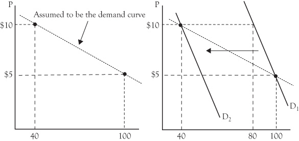
Figure 3.7. Incorrect inference of elasticity.

This suggests that demand is relatively elastic. Each 1% increase in the price led to a 1.28% decrease in the quantity demanded.
The graph on the right shows another possibility. One of the other determinants of demand may have changed; for example, the price of a substitute may have decreased. This would cause the demand curve to shift to the left. Had the price of the substitute remained unchanged, the quantity demanded would only have fallen to 80 units in response to the price increase. If so, the price elasticity coefficient would have been equal to:

This suggests that demand is relatively inelastic. Each 1% increase in the price only led to a 0.33% decrease in the quantity demanded.
Unfortunately, the manager does not observe the 80 units that would have been sold if the price had increased to $10 and the price of the substitute had not changed. Because the price of the substitute did change, he only observes the 40 units that are sold. This misleads him into thinking consumers are more price sensitive than they actually are. One should note that the scenario on the right is likely to be encountered more often than not. Managers usually do not change prices randomly. Most of the time, the price change was motivated by a change in a factor that can shift a demand curve, such as the price charged by competing firms.
The relationship between price elasticity and revenue is important. For example, suppose a firm raises its price from $5 to $10 and the quantity demanded falls from 100 units to 60 units. In this case, raising the price caused the firm’s revenue to increase from $500 to $600. Suppose, however, that in response to the price increase, the quantity demanded falls from 100 units to 40 units. In this circumstance, the price increase caused revenues to fall from $500 to $400. Figure 3.8 illustrates the distinction. Note that the demand curve that corresponds to the decrease in revenues is more elastic than the demand curve that is associated with an increase in revenues.

Figure 3.8. Elasticity and revenue.
When we reflect on the definitions of elastic and inelastic in Table 3.4, the relationship between elasticity and revenue should become fairly obvious. We define demand as “elastic” if the percentage change in quantity exceeds the percentage change in price. If, for example, the price rises by 10%, the quantity demanded will fall by more than 10%, which implies that revenue will decrease. If, on the other hand, the price declines by 10%, the quantity demanded will rise by more than 10%. This suggests that revenues will increase in response to the price cut. In general, when the demand is elastic, price and revenue will move in opposite directions.
If demand is relatively inelastic, the percentage change in the quantity demanded will be less than the percentage change in the price. Thus, if the price rises by 10%, the quantity demanded will fall by less than 10%, causing revenue to rise. If the price falls by 10%, the quantity demanded will rise by less than 10%, leading to a decrease in revenue. If demand is inelastic, therefore, price and revenue will move in the same direction.
Finally, if demand is unitary, a given percentage change in the price will lead to an identical percentage change in the quantity demanded. For example, a 10% price hike will lead to a 10% decline in the quantity demanded. The two percentage changes cancel out, causing revenues to remain the same. Table 3.5 summarizes the relationship between elasticity and revenue.
Table 3.5. Relationship Between Elasticity and Revenue
|
1. Elastic |
% change in QD > % change in P |
Price and revenue move in opposite directions |
|
2. Inelastic |
% change in QD < % change in P |
Price and revenue move in the same direction |
|
3. Unitary |
% change in QD = % change in P |
Revenue will not change if the price changes |
Apple Corporation’s iTunes illustrated the relationship between price elasticity and revenue when it increased the price of many of its songs from $.99 to $1.29 in 2009. One day after the price increase, 60 songs on its top 100 charts carried a price of $1.29 whereas the remaining 40 were still priced at $.99. In 24 hours, the $1.29 songs lost an average of 5.3 positions in the charts while the $.99 songs gained an average of 2.5 positions. The data revealed that the number of downloads for songs whose prices had been raised fell relative to those whose prices remained at $.99.
But did fewer downloads translate into more or less revenue? According to Nielsen Soundscan data, a #42 song is downloaded roughly 9,800 times over a two-day period.6 At a price of $.99, the song generates $9,702 over that time span. In contrast, a #45 song is downloaded approximately 9,200 times over two days. At a retail price of $1.29, the song generates $11,868 over two days. Hence, if raising the price from $.99 to $1.29 causes the number of downloads to fall from 9,800 to 9,200 over a two-day period, revenues rise by over $2,000. In general, downloads would have to drop by more than 23% for the price increase to cause revenues to fall.
Although many persons (economists included) tend to label a good as having either an elastic demand or an inelastic demand, the elasticity for a linear demand curve depends on the price. If we examine the demand schedule in Table 3.6 and calculate the price elasticity of demand between each pair of prices, the results are illuminating.
Table 3.6. Price Elasticities Along the Demand Curve

As Table 3.6 indicates, the price elasticity of demand is not constant across all prices. Between $3 and $5, demand is inelastic. Between $5 and $6, demand is unitary, and demand is elastic for prices above $6. We can also see that as we move up the demand curve, the coefficient becomes increasingly elastic.
This revelation should not be too surprising. We used snack foods at a convenience store to illustrate why the price of snack foods could be 50% higher than at a supermarket without causing sales to suffer dramatically. Let’s assume that the manager of the store increased the price of a candy bar from $.50 to $.75. Although the number of candy bars sold decreased revenues increased. This would indicate that the candy bars had an inelastic demand. The manager would be foolish to believe that candy bars would have an inelastic demand at all prices. If consumers were relatively insensitive to candy bar prices, and price increases were inevitably accompanied by rising revenue, then charging $25 for a candy bar would yield far greater revenues than $.75. Clearly, the store would be hard pressed to sell any candy bars at a price of $25. It stands to reason, then, that somewhere between $.75 and $25, the demand goes from being inelastic to elastic.
Let’s see how the relationship between elasticity and the demand curve affects relevant revenue. Theory suggests that demand tends to be relatively inelastic at lower prices, becomes unitary at a higher price, and eventually becomes elastic at even higher prices. Earlier, we stated that if the current price is in the inelastic portion of a demand curve, an increase in the price will cause revenues to rise. On the other hand, if the current price is in the elastic section of the demand curve, decreasing the price will cause revenues to rise. Understanding price elasticity is clearly important when one attempts to estimate the relevant revenue associated with a price change.
However, we can take theory one step further. If price increases in the inelastic section cause revenue to rise, and price cuts in the elastic section also cause revenue to rise, the firm will maximize revenues by setting its price in the unitary section of the demand curve. This is shown in Figure 3.9. As the price moves toward P*, revenues rise. Total revenues are maximized by setting the price in the unitary section of the demand curve. At that price, Q* units are demanded.

Figure 3.9. Elasticity and the revenue-maximizing price.
Of course, firms are interested in maximizing profits, not revenues. Although an understanding of price elasticity is critical to the decision maker, the scenario exhibited in Figure 3.9 will also maximize profits if the firm has no variable costs. This is likely to be the case for setting ticket prices. The seats already exist; the relevant decision is what price to charge. Because variable costs will not change as more tickets are sold, the firm seeks the ticket price that will maximize revenues. In doing so, it will also maximize profits. Note that in this context, the ticket seller may actually be more profitable by leaving seats empty than by lowering the price to assure a sellout.
Cross-Price Elasticity of Demand
Another concept that is critical to anticipating relevant revenue is the cross-price elasticity of demand. Often, a firm may offer complementary or substitute goods in its product lines. At Burger King, French fries and soft drinks are complements to hamburgers. Proctor and Gamble’s line of laundry detergents include Tide, Cheer, and Bold. Although they are all P&G brands, consumers view them as substitutes. When a firm has product lines that serve as either complements or substitutes for other lines, a change in the price of one good might affect the unit sales of the other good. An increase in the price of hamburgers at Burger King may decrease not only the quantity of hamburgers demanded, but also the quantity of fries demanded. This is illustrated in Figure 3.10.
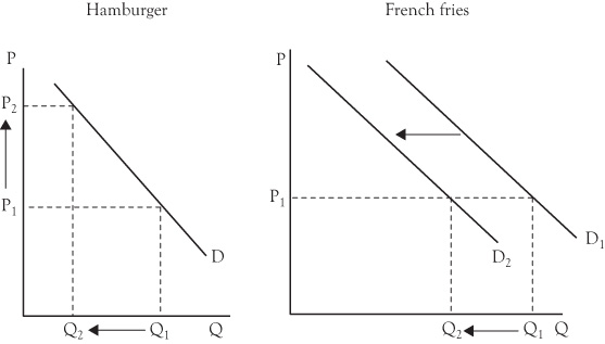
Figure 3.10. Cross-price elasticity of demand.
The cross-price elasticity of demand is a means to measure the sensitivity of unit sales of one good to changes in the price of a related good. It is calculated as:
EC = % change in the quantity of good Y purchased/% change in the P of good X,
where goods X and Y are either substitutes or complements. In evaluating the coefficient, the primary difference between the cross-price elasticity of demand and the standard price elasticity coefficient is that the latter is, by definition negative (price and quantity are inversely related on the demand curve). Therefore, economists usually ignore the negative sign. In contrast, the cross-price elasticity of demand can be either positive or negative, depending on the relationship between X and Y. If the two goods are complementary, an increase in the price of X will cause the unit sales of Y to fall, implying a negative cross-elasticity coefficient. For example, if the estimated cross-elasticity coefficient is –3, a 1% increase in the price of X will lead to a 3% decrease in the unit sales of the complementary product. If X and Y are substitutes, an increase in the price of X will result in increased unit sales of Y. In this case, the cross-elasticity coefficient will be positive. As an example, a cross-elasticity coefficient of 0.85 implies that a 1% increase in the price of X will cause the unit sales of the substitute good, Y, to increase by 0.85%.
The cross-elasticity coefficient can be useful to determine the degree of complementarity or substitutability across product lines. Suppose, for example, that the cross-elasticity coefficient that measures the responsiveness of French fry sales to changes in hamburger prices is –4. In contrast, suppose the coefficient that measures the responsiveness of ice cream sundaes to changes in hamburger prices is –0.10. The first scenario implies that each 1% increase in the price of hamburgers decreases the quantity of French fries sold by 4% whereas, in the second case, a 1% increase in the price of hamburgers causes ice cream sundae sales to fall by 0.10%. Together, these coefficients imply that fries are a much closer complement to hamburger sales than are ice cream sundae sales.
The same type of comparisons can be made for product lines that are potentially substitutes for each other. The cross-elasticity coefficient that measures the responsiveness of chicken sandwich sales to changes in hamburger prices may be 1.5, whereas the responsiveness of salad sales to changes in hamburger prices may be 0.3. One would infer from these coefficients that chicken sandwiches are considered by customers to be closer substitutes for hamburgers than salads.
In anticipating relevant revenue, firms need to be cognizant of how a price/production decision for one good might affect the unit sales of related goods in their product lines. If the firm lowers the price for one good, the increase in unit sales will be accompanied by rising unit sales in complementary goods. Hence, the relevant revenue would be equal to the sum of the output and price effects for the product whose price has changed, plus the additional revenue generated for its complement.
On the other hand, if the product line includes substitutes, the relevant revenue from a price cut will be less than the marginal revenue from the good in question. Any price decrease aimed at increasing unit sales for one good will cannibalize some of the unit sales for the substitute good in the firm’s product line. Hence, the relevant revenue will be the sum of the output and price effects for the good in question less the loss in revenue from declining unit sales for the substitute good.
Summary
•The law of demand states that as the price of a good rises, the quantity demanded decreases. This means that to sell more units, firms will have to lower prices.
•The relevant revenue in production decisions is called marginal revenue. Marginal revenue associated with a production increase is the sum of the output and price effects. The output effect is the revenue generated by the additional units sold. The price effect is the lost revenue due to dropping the price on the other units.
•Changes in other factors can cause demand to increase or decrease. Changes in incomes, prices of substitutes, prices of complementary goods, consumer tastes, and price expectations may allow the firm to sell more units or fewer units at the same price.
•Price elasticity measures the responsiveness of the quantity demanded to changes in the price. If the percentage change in the quantity demanded exceeds the percentage change in the price, demand is elastic. If the percentage change in the quantity demanded is less than the percentage change in the price, demand is inelastic. If the percentage change in the quantity demanded is equal to the percentage change in the price, demand is unitary.
•Price elasticity is determined by whether the good is a luxury or a necessity, the availability of substitutes, the definition of the market, the price of the good as a percentage of the buyer’s budget, and the time the buyer has to make a purchase.
•Price elasticity is measured as: (New quantity – old quantity)/(average of the quantities) divided by (New price – old price)/(average of the prices). The coefficient reports the percentage change in the quantity demanded resulting from a 1% change in the price. If the ratio exceeds 1, demand is elastic. If the ratio is less than 1, demand is inelastic. If the ratio is equal to 1, demand is unitary.
•The higher the price of the good, the more elastic the demand. At lower prices, demand is inelastic. As the price rises, demand becomes unitary. As the price continues to rise, demand becomes elastic. Revenues are maximized by setting the price in the unitary section of the demand curve.
•The cross-elasticity of demand measures the responsiveness of the quantity demanded of one good to price changes in a related good. In terms of relevant revenues, firms should be cognizant as to how price changes will affect the unit sales of substitute or complementary goods in their product line.