Chapter 10: Presenting Output and Project Disposition
Synthesis - Review and Approach
Algorithms: Presenting Selected Measurements of Utilization, Cost to Medicare, and Quality Outcomes
Presenting Ambulance Utilization
Presenting Medicare Payments for Evaluation and Management Services by Provider
Presenting Rates of Diabetes and COPD
Algorithms: Presenting Inpatient Length of Stay Information by State
Algorithms: Presenting Mean Medicare Part A Payments per Beneficiary by State and County
Algorithms: Presenting Rates of Diabetic Eye Exams
Archiving Materials for Future Use
It has been a long a journey! We learned about the Medicare program, Medicare data, and knocked out all but the final steps in our example research programming project. The purpose of this chapter is to take the final steps in our research programming project by synthesizing our results and completing the project disposition phase of our project plan. As discussed in earlier chapters, the online companion to this book is at http://support.sas.com/publishing/authors/gillingham.html. Here, you will find information on creating dummy source data, the code in this and subsequent chapters, as well as answers to the exercises in this book. I expect you to visit the book’s website, create your own dummy source data, and run the code yourself.
At this point in our project, it is easy to think we are nearly finished! After all, we performed some serious data manipulation to create analytic files for enrollment, utilization, and cost analyses, including looking at chronic conditions and quality measurement. We positioned our project well; all we need to do is deliver some output, right? Well, not so fast! By now, you probably realize that nothing is as easy as it first appears! As investigators, we need to put a lot of thought into presenting the information stored in our analytic files in a meaningful way. Then, after presenting our results, we must close out the project. The process of ending a project methodically is called project disposition; disposition requires ample time and effort to ensure that our specifications, code, and results will be clear to us for years to come. In this way, the proper disposition of our example research programming project brings an extra layer of legitimacy to our work, and facilitates our ability to use our work in the future.
Before we begin, instead of our usual review of topics relevant to our programming work, we will reward ourselves by reviewing all of our fantastic accomplishments! Recall that we have undertaken an effort to evaluate the effectiveness of a pilot program that is designed to incentivize providers to reduce costs to Medicare and improve quality outcomes. Our evaluation effort hinges on measuring utilization, cost to Medicare, and quality by using a list of beneficiaries who interacted with the providers in our sample population; recall that this list of providers and beneficiaries was provided to us at the outset of our study. To these ends, we performed the following work:
• In Chapters 4 and 5, we established our project plan. In addition, we requested, received, loaded, and transformed the data used in subsequent chapters.
• In Chapter 6, we created a file that contained demographic information for beneficiaries who were continuously enrolled in Medicare FFS throughout all twelve months of calendar year 2010.
• In Chapter 7, we created analytic files that contained summaries of utilization of services for our population of continuously enrolled beneficiaries.
• In Chapter 8, we created analytic files that contained summaries of the costs to Medicare for services for our population of continuously enrolled beneficiaries.
• In Chapter 9, we identified beneficiaries with diabetes or COPD. In addition, we created analytic files that focused on simple measurements of quality outcomes.
Until now, our programming adventure has focused on calculating the information needed to answer the research questions we posed at the beginning of our example project. Now, we must slightly shift our focus to finish our work by presenting our utilization, cost, and quality outcome measurements. To this end, we will utilize data from some of the analytic files that we created in prior chapters, and use some of the work that we performed in Chapter 6 to add state and county names to our file of continuously enrolled beneficiaries.
The algorithms that we will develop in the chapter are by no means exhaustive, and we do not endeavor to summarize all of the analyses that we computed in prior chapters. We could think of many, many additional ways of looking at the output we created. For example, we could present analyses of outcomes that are broken out by provider specialty; we could compare the measurements for the population of providers in our finder file against other providers that did not participate in the program we are studying; or, we could compare results over time to look for significant changes in outcomes. The purpose of this text is to lay the groundwork for the reader to be able to independently answer these questions. Therefore, one of the chapter exercises listed below asks you to think of some additional questions we might answer with our data.
Let’s start by simply displaying the following pieces of our utilization, cost to Medicare, and quality outcomes of the work that we performed in Chapter 7 through Chapter 9, respectively:
• Drawing on our work in Chapter 7, we will present ambulance utilization information by beneficiary age.
• Drawing on our work in Chapter 8, we will present Medicare payments for E&M services summarized by the providers in our study population.
• Drawing on our work in Chapter 9, we will present rates of diabetes and COPD in our population of continuously enrolled beneficiaries.
Again, we could have easily chosen to present other information that we calculated in previous chapters, like the total costs to Medicare that were associated with home health agency services. One of the chapter exercises listed below asks you to choose and present information that was calculated in Chapter 7, Chapter 8, or Chapter 9 other than what was chosen as an example for our work in this section.
One interesting presentation of output is to examine beneficiaries with at least one claim for ambulance services, along with the age of each beneficiary. This type of algorithm provides a good example for analyzing relevant summary information that may be used to guide further analyses.
In Step 10.1, we begin our work to present ambulance utilization information by merging our file of continuously enrolled beneficiaries (ENR.CONTENR_2010_FNL) with the analytic summary file UTL.AMB_UTIL created in Step 7.11 of Chapter 7 (we also bring in our formatting of age categories that you will recognize from our work in Chapter 6). The file UTL.AMB_UTIL contains one record per beneficiary with at least one claim for an ambulance service. Because both files are already sorted by BENE_ID, there is no need for a pre-merge sort. The outputted file, called FNL.PRESENT_AMB, contains one record for each of the beneficiaries in UTL.AMB_UTIL (we use an “if b” merge), as well as the STUDY_AGE and AGE_CATS variables (kept from the ENR.CONTENR_2010_FNL file) and the TOT_AMB_SVC variable (kept from the ambulance utilization analytic file).
/* STEP 10.1: MERGE CONTINUOUSLY ENROLLED BENEFICIARIES WITH AMBULANCE UTILIZATION DATA */
proc format;
value age_cats_fmt
0='AGE LESS THAN 65'
1='AGE BETWEEN 65 AND 74, INCLUSIVE'
2='AGE BETWEEN 75 AND 84, INCLUSIVE'
3='AGE BETWEEN 85 AND 94, INCLUSIVE'
4='AGE GREATER THAN OR EQUAL TO 95';
run;
data fnl.present_amb(keep=bene_id tot_amb_svc study_age age_cats);
merge enr.contenr_2010_fnl(in=a) utl.amb_util(in=b);
by bene_id;
if b;
run;
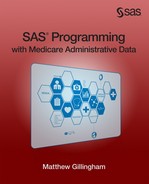
Next, in Step 10.2, we use ODS to present a PROC SUMMARY of the beneficiaries with at least one claim for an ambulance service (using a ‘where’ clause that the value of TOT_AMB_SVC is not null), along with the number of ambulance services (the value of the TOT_AMB_SVC variable) and the beneficiary’s age category (the value of AGE_CATS). Note that we must first sort the file by AGE_CATS, and we utilize the formatting of the AGE_CATS variable in our presentation of the output.
/* STEP 10.2: PRESENT MEASUREMENT OF AMBULANCE UTILIZATION */
proc sort data=fnl.present_amb;
by age_cats;
run;
ods html file=“C:UsersmgillinghamDesktopSAS BookFINAL_DATAODS_OUTPUTGillingham_fig10_2.html”
image_dpi=300 style=GrayscalePrinter;
ods graphics on / imagefmt=png;
title “LISTING OF BENEFICIARIES WITH AMBULANCE UTILIZATION GROUPED BY AGE_CATS”;
proc summary data=fnl.present_amb(where=(tot_amb_svc ne .)) print;
var tot_amb_svc;
by age_cats;
format age_cats age_cats_fmt.;
run;
ods html close;
Output 10.1 is a snapshot of some of the output of Step 10.2.
Output 10.1: List of Beneficiaries with Ambulance Utilization Grouped by AGE_CATS
Another interesting presentation of the summary analytic files created in previous chapters is a listing of summary statistics related to costs to Medicare for evaluation and management visits. In this example, we use the file that contains providers and their associated beneficiaries (described in Chapter 5 as our “finder file” or “attribution file”) in our analysis. Recall we received this file at the beginning of our example research programming project, and we used it to guide our project’s data extraction process. Now, we use this attribution file to examine costs for the sample of providers in our study.
We measured total E&M costs to Medicare using the code presented in Step 8.2 of Chapter 8, outputting a data set called CST.EM_CST_BENE that contains one record for each beneficiary, along with a variable called EM_TOTCOST_BENE that is a summary of each beneficiary’s total E&M costs. Now, in Step 10.3, we merge the CST.EM_CST_BENE data set with our attribution file (called SRC.FINDER_ATTRIB) in order to “attribute” a provider to each beneficiary in the E&M cost summary data set. Both data sets are already sorted by BENE_ID, so pre-merge sorting is not necessary. We keep only those records in the CST.EM_CST_BENE data set (i.e., we perform an “if b” merge) because those are the beneficiaries for whom we have E&M cost information. We output a data set called PRESENT_EMCOST that contains the E&M cost information (EM_TOTCOST_BENE) for each continuously enrolled beneficiary with at least one E&M service, as well as the identifier variable of the provider associated with that beneficiary (PRFNPI).
/* STEP 10.3: MERGE E&M COST INFORMATION WITH PROVIDER ATTRIB FILE */
data present_emcost(keep=bene_id prfnpi em_totcost_bene);
merge src.finder_attrib(in=a) cst.em_cost_bene(in=b);
by bene_id;
if b then output present_emcost;
run;
Finally, in Step 10.4, we use PROC SQL to summarize the E&M cost information (EM_TOTCOST_BENE) contained in the FNL.PRESENT_EMCOST data set by provider (PRFNPI).We call our summarized cost EM_TOTCOST_PROV. We also summarize the number of relevant beneficiaries into a variable called EM_TOTBENE_PROV. We output a file called FNL.PRESENT_EMCOST.
/* STEP 10.4: PRESENT MEASUREMENT OF E&M COSTS TO MEDICARE BY PROVIDER */
proc sql;
create table fnl.present_emcost as
select prfnpi, count(distinct bene_id) as em_totbene_prov, sum(em_totcost_bene) as
em_totcost_prov format=dollar15.2 label='TOTAL E&M COST FOR PROVIDER'
from present_emcost
group by prfnpi;
quit;
Output 10.2 is a snapshot of some of the output of Step 10.4, displayed in descending order by EM_TOTBENE_PROV.
Output 10.2: PROC PRINT of EM Costs to Medicare, Summed by Provider

Finally, let’s utilize our work that identified beneficiaries with diabetes or COPD by studying rates of these conditions in our population of continuously enrolled beneficiaries. This exercise provides a good example of presenting results that provide a framework for additional analyses. For example, if there are a small number of beneficiaries with diabetes in our overall population, the population of a particular county or state, or a population of beneficiaries attributed to a certain provider, we could surmise that some utilization and cost measurements may follow suit.
In Step 10.5, we begin our look at rates of diabetes and COPD in our population of continuously enrolled beneficiaries by merging our file containing a list of beneficiaries with COPD or diabetes with our population of continuously enrolled beneficiaries. In Step 9.1 through Step 9.4 presented in Chapter 9, we created a file called CND.DIA_COPD_COND. This file contains one record per beneficiary with either diabetes or COPD (or both diabetes and COPD). Because this data set contains records only for beneficiaries with diabetes or COPD, we must merge the file with our population of continuously enrolled beneficiaries to learn about the number of beneficiaries with diabetes or COPD in our population as a whole. To this end, we merge the CND.DIA_COPD_COND data set with the same ENR.CONTENR_2010_FNL data set used above, keeping all records in the ENR.CONTENR_2010_FNL data set to create the data set FNL.PRESENT_DIACOPD. The values of the variables identifying beneficiaries with diabetes or COPD in the data set CND.DIA_COPD_COND are set equal to zero for beneficiaries in ENR.CONTENR_2010_FNL who are not in CND.DIA_COPD_COND (indicating that these beneficiaries were not identified as having diabetes or COPD).
/* STEP 10.5: MERGE CONTINUOUSLY ENROLLED BENEFICIARIES WITH POPULATION OF DIABETICS AND BENES WITH COPD */
data fnl.present_diacopd(keep=bene_id dia_flag copd_flag);
merge enr.contenr_2010_fnl(in=a) cnd.dia_copd_cond(in=b);
by bene_id;
if a;
if dia_flag=. then dia_flag=0; if copd_flag=. then copd_flag=0;
run;
In Step 10.6, we present a simple frequency distribution of beneficiaries with diabetes or COPD (or both diabetes and COPD) using a PROC FREQ of the data set FNL.PRESENT_DIACOPD that we created in Step 10.5. We perform frequency distribution on the variable that identifies beneficiaries with diabetes (DIA_FLAG) and the variable that identifies beneficiaries with COPD (COPD_FLAG). In addition, we perform a cross-tabulation of these variables. As in previous examples in this chapter, we use ODS to output the PROC FREQ results to the same folder where our permanent data is stored for our work in this chapter.
/* 10.6: PRESENT RATES OF DIABETES, COPD, AND BOTH DIABETES AND COPD */
ods html file=“C:UsersmgillinghamDesktopSAS BookFINAL_DATAODS_OUTPUTGillingham_fig10_6.html”
image_dpi=300 style=GrayscalePrinter;
ods graphics on / imagefmt=png;
title “RATES OF DIABETES AND COPD IN CONTINUOUSLY ENROLLED BENEFICIARY POPULATION”;
proc freq data=fnl.present_diacopd;
tables dia_flag copd_flag / missing;
run;
ods html close;
Output 10.3 shows the results of Step 10.6.
Output 10.3: Rates of Diabetes and COPD in Continuously Enrolled Beneficiary Population

In this section, we build on our work presenting the work of previous chapters by displaying the inpatient length of stay by state. To this end, we use the data set UTL.STAY_UTL that we created in Step 7.5 through Step 7.8 presented in Chapter 7. This data set contains summary information on length of stay, but it also contains one record for each beneficiary’s unique inpatient claim admission and discharge dates (more on this below). We also use the data set of continuously enrolled beneficiaries used in the examples above. This data set, called ENR.CONTENR_2010_FNL, contains information on each beneficiary’s state of residence (added to the ENR.CONTENR_2010_FNL data set in Chapter 6).
As mentioned above, the UTL.STAY_UTL data set contains one record for each beneficiary’s unique inpatient claim admission and discharge dates. We do not need to use the admission and discharge date information for our analysis. Therefore, in Step 10.7, we sort the UTL.STAY_UTIL data set, removing duplicate records for each beneficiary, and keeping only the beneficiary identifier and summary information pertaining to each beneficiary’s hospital stays. The output, a data set called STAY_UTIL, contains one record for each beneficiary, as well as each beneficiary’s inpatient length of stay summary information.
/* STEP 10.7: REMOVE STAY DATES AND SORT IP STAY UTILIZATION DATA */
proc sort data=utl.stay_util(keep=bene_id stay_cnt tot_ip_los ip_alos) out=stay_util nodupkey;
by bene_id;
run;
In Step 10.8, we add the name of the beneficiary’s state to the STAY_UTIL data by merging it with the ENR.CONTENR_2010_FNL data set. We are presenting a summary of length of stay only for those beneficiaries with at least one inpatient claim, so we do not retain all beneficiaries in the ENR.CONTENR_2010_FNL data set (i.e., we use an “if b” merge to ensure we retain only the beneficiaries with at least one hospital stay). We call the output of this merge FNL.PRESENT_IPLOS.
/* 10.8: MERGE INPATIENT LENGTH OF STAY DATA WITH BENEFICIARY SSA STATE INFORMATION */
data fnl.present_iplos(keep=bene_id stay_cnt tot_ip_los ip_alos state);
merge enr.contenr_2010_fnl(in=a) stay_util(in=b);
by bene_id;
if b;
run;
In Step 10.9, we sort the FNL.PRESENT_IPLOS data set in preparation for displaying data by state. Specifically, we sort the FNL.PRESENT_IPLOS by the variable STATE, which will be the ‘by’ variable in the PROC FREQ performed in the next step.
/* STEP 10.9: SORT DATA BY SSA STATE IN PREPARATION FOR PRESENTATION OF IP LOS BY SSA STATE AND COUNTY */
proc sort data=fnl.present_iplos;
by state;
run;
Finally, in Step 10.10, we perform a PROC FREQ to output measurement of the average inpatient length of stay for each beneficiary (IP_LOS), by the name of the state (STATE) associated with the beneficiary’s SSA state code provided in the MBSF data. Once again, we use ODS to output the PROC FREQ results to the same folder where our permanent data is stored for our work in this chapter. Note that we limit our frequency to the state of Michigan, and to values of IP_ALOS that are between 1 and 5 days.
/* STEP 10.10: PRESENT IP LOS INFORMATION BY BENEFICIARY SSA STATE */
ods html file=“C:UsersmgillinghamDesktopSAS BookFINAL_DATAODS_OUTPUTGillingham_fig10_10.html”
image_dpi=300 style=GrayscalePrinter;
ods graphics on / imagefmt=png;
title “FREQUENCY OF IP LOS BY SSA STATE”;
proc freq data=fnl.present_iplos(where=(state='MI' and 1<=ip_alos<=5));
tables ip_alos;
by state;
run;
ods html close;
Output 10.4 shows the output of Step 10.10.
Output 10.4: Frequency of IP LOS by SSA State

Understanding the landscape of costs to Medicare adds an important dimension to our analyses. For example, if our population contains many beneficiaries identified as having COPD, we might expect payments made by Medicare to be higher for this study population. In addition, understanding total costs to Medicare for the beneficiaries in our study population by geographic region opens the gateway to further analyses. For example, we could combine some of the techniques developed in these steps and apply them to a study of total costs to Medicare by chronic condition, or by provider in our study population.
In Step 10.11, we add beneficiary state and county information to our data set of total Part A costs to Medicare. This data set containing summary information on costs, called CST.PA_TOTCOST_BENE, was created in Chapter 8. Our merge to add state and county information to this data set looks the same as the merge presented in Step 10.8, except that we retain all records in the ENR.CONTENR_2010_FNL data set (i.e., we perform an “if a” merge). In addition, we add a line of code to set the value of the variable summarizing total Part A costs to Medicare (PA_TOTCOST_BENE) equal to 0 for beneficiaries without a record in the ENR.CONTENR_2010_FNL data set because it is possible (though unlikely) for a beneficiary to have an enrollment record without any corresponding claims. The output of this merge, a data set called FNL.PRESENT_PACOST, contains one record for each continuously enrolled beneficiary, along with each beneficiary’s total Part A cost summary information, and information on the beneficiary’s state and county of residence.
/* 10.11: MERGE TOTAL PART A COST DATA WITH BENEFICIARY SSA STATE AND COUNTY INFORMATION */
data fnl.present_pacost(keep=bene_id pa_totcost_bene state county);
merge enr.contenr_2010_fnl(in=a) cst.pa_totcost_bene(in=b);
by bene_id;
if a;
if a and not b then pa_totcost_bene=0;
run;
In Step 10.12, we sort the output of Step 10.11 by STATE and COUNTY in preparation for displaying total Part A costs to Medicare by STATE and COUNTY in the PROC MEANS presented in the next step.
/* STEP 10.12: SORT DATA BY SSA STATE AND COUNTY IN PREPARATION FOR PRESENTATION OF COST BY SSA STATE AND COUNTY */
proc sort data=fnl.present_pacost;
by state county;
run;
Finally, in Step 10.13, we perform a PROC MEANS on our summaries of total Part A costs to Medicare in order to present mean Medicare payments per beneficiary by state and county name. As in the prior example, we use ODS to output the results to the same folder where our permanent data is stored for our work in this chapter, and we limit the output to those beneficiaries who reside in a single county in Michigan. We also ask for the minimum and maximum values for each state and county combination.
/* STEP 10.13: PRESENT TOTAL PART A COST BY BENEFICIARY SSA STATE AND COUNTY */
ods html file=“C:UsersmgillinghamDesktopSAS BookFINAL_DATAODS_OUTPUTGillingham_fig10_13.html”
image_dpi=300 style=GrayscalePrinter;
ods graphics on / imagefmt=png;
title “PROC MEANS OF TOTAL PART A COST TO MEDICARE BY SSA STATE AND COUNTY”;
proc means data=fnl.present_pacost(where=(state='MI' and county='WASHTENAW'))
n nmiss mean min max maxdec=1;
var pa_totcost_bene;
by state county;
run;
ods html close;
Output 10.5 shows the results of Step 10.13, delimited to print for one county in Michigan.
Output 10.5: PROC MEANS of Total Part A Cost to Medicare by SSA State and County

In our final example, we present the occurrence of diabetic eye exams by SSA state and county name. We wish to limit our presentation only to those continuously enrolled beneficiaries who are identified as diabetic. This work incorporates the work of previous chapters to identify beneficiaries who have diabetes, and then requires us identify diabetic eye exam services for these diabetic beneficiaries.
Specifically, we utilize the data set CND.EYE_DIA_COND that we created in Chapter 9 and use the variable EYE_SVC, which flags evidence that a diabetic beneficiary has had a service for a diabetic eye exam. However, the data set CND.EYE_DIA_COND contains records only for beneficiaries identified as having a diabetic eye exam. Because we want to look at the occurrence of diabetic eye exams in the overall population of continuously enrolled beneficiaries identified as diabetic, we must utilize the data set CND.DIA_COPD_COND that contains a list of beneficiaries identified as having diabetes. Finally, we utilize the ENR.CONTENR_2010_FNL data set to add beneficiary state and county name information to our analysis.
To this end, in Step 10.14, we perform a merge as follows:
• We merge three data sets (CND.EYE_DIA_COND, CND.DIA_COPD_COND, and ENR.CONTENR_2010_FNL).
• Using the data set CND.DIA_COPD_COND, we set the population of our output file to be only those continuously enrolled beneficiaries who were identified as having diabetes.
• We use the data set CND.EYE_DIA_COND to add the EYE_SVC flag to the output data set.
• We use the data set ENR.CONTENR_2010_FNL to add HRR information for each beneficiary in the output data set.
• We output a data set called FNL.PRESENT_EYEDIA, keeping the state and county name variables (STATE and COUNTY), as well as the EYE_SVC variable. Note that the missing values of EYE_SVC (created for those continuously enrolled beneficiaries with diabetes who did not receive a diabetic eye exam) are set equal to zero.
/* STEP 10.14: MERGE CONTINUOUS ENROLLMENT AND DIABETIC EYE EXAM INFORMATION */
data fnl.present_eyedia(keep=bene_id eye_svc state county);
merge enr.contenr_2010_fnl(in=a) cnd.eye_dia_cond(in=b) cnd.dia_copd_cond(in=c keep=bene_id dia_flag);
by bene_id;
if c and dia_flag=1;
if eye_svc=. then eye_svc=0;
run;
In Step 10.15, we sort the output of Step 10.14 by STATE and COUNTY in preparation for displaying the number of diabetic eye exams by STATE and COUNTY in the PROC FREQ presented in the next step.
/* STEP 10.15: SORT DATA BY SSA STATE AND COUNTY IN PREPARATION FOR PRESENTATION BY SSA STATE AND COUNTY */
proc sort data=fnl.present_eyedia;
by state county;
run;
Finally, in Step 10.16, we perform two separate PROC FREQs on the EYE_SVC variable. First, we create a frequency distribution of the rates of diabetic eye exams in the overall population of continuously enrolled beneficiaries with diabetes. Next, we perform the same frequency distribution by STATE and COUNTY, limiting our analysis to a single county in Michigan. You can see that there are few beneficiaries in the overall population who did not receive a diabetic eye exam, and there are no beneficiaries in Washtenaw County Michigan who did not receive a diabetic eye exam. We use ODS to output the results to the same folder where our permanent data is stored for our work in this chapter.
/* STEP 10.16: PRESENT MEASUREMENT OF DIABETIC EYE EXAM SERVICES BY OVERALL AND BY SSA STATE AND COUNTY */
ods html file=“C:UsersmgillinghamDesktopSAS BookFINAL_DATAODS_OUTPUTGillingham_fig10_16.html”
image_dpi=300 style=GrayscalePrinter;
ods graphics on / imagefmt=png;
title “RATES OF DIABETIC EYE EXAMS”;
proc freq data=fnl.present_eyedia;
tables eye_svc / missing;
run;
proc freq data=fnl.present_eyedia(where=(state='MI' and county='WASHTENAW'));
tables eye_svc / missing;
by state county;
run;
ods html close;
Output 10.6 shows the results of Step 10.16.
Output 10.6: Rates of Diabetic Eye Exams

As stated below, all programs should be executed in batch mode such that the logs and lists have the same name as their parent program (but a different file extension, of course). In addition, it is helpful to undertake a “production” execution of the code that entails running each program in sequence without breaks so that the date and time stamps on the files are sequential. Depending on your operating system, executing code in batch can be as simple as “right clicking” on the file you wish to execute and selecting the option to execute in batch. Upon completion, log and list files are generated automatically. The reader should carefully review the logs for errors, warnings, and uninitialized variables (this can be accomplished quite easily by performing a find on “error,” “warning,” and “uninitialized”. If the reader is operating in a UNIX environment, he or she can execute a script in the UNIX shell to execute the code in batch. Prior to executing in batch, I strongly recommend that the reader either delete data sets created during the code development and testing process, or work in a production partition of the system that does not contain data sets created during the development and testing process. The reason this step is strongly recommended is that it is remarkably easy to accidentally input a development data set (that may contain incorrect information) in your production run. As long as your code is pointing to an existing data set, SAS will input and use the data set that the code is pointing to regardless of whether or not you intend for it to do so.
Now that we have completed all of our programming, it is time to end our project. The disposition phase of the project is just as important as any other part of our work. As we discussed in Chapter 4, project disposition involves creating a “package” that will stand the test of time, documenting our work for future reference. In addition, because our project uses personally identifiable Medicare data, project disposition also includes the destruction of project data as specified in our Data Use Agreement (DUA). Should we perform this task improperly, we may not be able to turn to our work for future reference (which would be a real shame, considering all of the hard work we put into it!). Even more importantly, the consequence of not adhering to our DUA is something we do not dare to contemplate!
Believe me, I have been here plenty of times. At this point in the project, you are probably very tired of the subject matter, as you have been toiling over a specific set of research questions and writing code. Nothing sounds better than to shut down your computer and go take a nap! I should warn you, however, that if you walk away now, you would be sorry. Picture this: Your fearless author, about one year after completing my first research programming project, is searching my hard drive in frustration for an algorithm I know is just perfect for my current project. Unfortunately, that algorithm is nowhere to be found, lost to time and buried in a jungle of files on my hard drive! You can learn from my mistakes by reading the remainder of this chapter and thinking about the best way to archive your work so it becomes a future resource, and not a source of frustration.
Our goal boils down to something quite simple; document and save the work we just completed in a way that enables us to utilize it for future work. In addition, CMS owns the code, logs, lists, technical documentation, and data created for any project funded by CMS, so archiving may involve additional work to transmit our archived materials to CMS. The following steps go a long way to completing our archiving goal:
• All programs should contain complete inline documentation, and should be clearly named so they sort in the order in which they run. For example, our code could be separated into distinct programs named 05_ETL.sas (the work performed to load our data performed in Chapter 5), 06_Enrollment.sas (the enrollment work performed in Chapter 6), 07_Utilization.sas (the utilization work performed in Chapter 7), and so on.
• All programs should be executed in batch mode so the logs and lists have the same name as their parent program. In addition, it is helpful to undertake a “production” execution of the code that entails running each program in sequence without breaks so that the date and time stamps on the files are sequential.
• All programs should be accompanied by technical documentation. Depending on your needs, technical documentation can be as simple as maintaining a listing of each program and its purpose, but as complex as an explanation of the purpose of every step in each program and including flow diagrams. Much of this book could be considered very comprehensive technical documentation for our code.
• All output should be labeled clearly and saved with meaningful filenames.
• All programs, logs, lists, technical documentation, and relevant output should be copied onto a CD-ROM or a DVD, being certain to follow the guidelines of our DUA. Including a “readme” file is helpful for documenting all of the files included on the storage media. It is important to keep in mind that the mere act of burning our files onto storage media does not guarantee that they will be preserved for time immemorial. Discs get scratched and hard drives break, so making a backup is highly recommended when contemplating long term storage of your work.
Most DUAs require the destruction of all Personally Identifiable Information (PII) data and some additional materials derived from PII data, even if those materials do not contain PII data themselves. Therefore, the first step in destroying data is to become clear on exactly what data must be destroyed. At the least, we must destroy all files containing PII. For our example research programming project, we will destroy all SAS data sets. Next, we must choose a method to destroy the data. The reader should check the details of his or her DUA. Common methods of destruction include shredding CDs or DVDs, erasure via degaussing of magnetic storage media such as hard drives, and deleting data stored on hard drives, followed by overwriting the deleted files many times to ensure they cannot be recovered.
In this chapter, we closed out our project by performing the following tasks:
• We used the files created in Chapters 5 through 10 to present the results of our study.
• We discussed the process for undertaking a final batch execution of all of our programs.
• We discussed the execution of the disposition of our project by documenting and archiving project materials for future use and destroying our data per the project’s Data Use Agreement.
1. What additional research questions might you answer with the data created in Chapter 5 through Chapter 9? Can you select and present calculations in Chapter 7, Chapter 8, or Chapter 9 that were not chosen as an example for our work in this chapter (e.g., rates of chronic conditions by age or sex)?
2. This text studied a pilot program that was operational during calendar year 2010. Updating a study annually is a fairly common exercise in health services research. Therefore, perform a thought experiment based on imagining what we would need to change in this text if the pilot program was operated during calendar year 2015.