
Chapter 8: Measuring Costs to Medicare
Review: Basics of Medicare Cost
A Note on Payment Standardization and Risk Adjustment
Algorithms: Measuring Evaluation and Management Payments
Algorithms: Measuring Inpatient Hospital Payments
Algorithms: Measuring Total Part A Payments
Measuring cost is important because it gets to the heart of the sustainability of any insurance program, and Medicare is certainly no exception. It is no understatement to say that the measurement of cost in the Medicare program is a hot topic. Open any newspaper or magazine or turn on the evening news and you will see that reducing cost without negatively affecting quality of care is the order of the day. In other words, the mission is to monitor and improve the value of purchased healthcare. To play a part in accomplishing this mission, we must learn how to measure the cost of care. In addition, we must learn to measure the quality of care, which we will do in Chapter 9 as we look at chronic conditions.
Utilization and quality are intimately linked to cost, but not always in ways one might assume. In your research, you may wish to go beyond simple measurements of utilization and cost and actually define categories of services whose payments may have been reduced by an incentive program. For example, did a program reduce the number of hospital stays, thus reducing total cost per beneficiary? Alternatively, did a program reduce the number of annual checkups, resulting in higher costs driven by an increase in the number of hospital stays?
In this text, the term “cost” is limited to the cost of the service to Medicare. We will not study the total cost of services, which include costs to beneficiaries, like coinsurance and deductibles. We are not studying services not covered by Medicare, like cosmetic surgery. In addition, because we retained only claims for acute short-stay hospitals in our inpatient data, we are not including payments for some services, like inpatient rehabilitation. Wrangling with all of these issues is beyond the scope of this introductory text, but it is important for readers to begin to think about these issues and prepare to account for them (or study them!) in their own research work. Rather, we utilize the Medicare payment variables in our claims data sets (i.e., the amount paid by the Medicare program to the provider for the services rendered) to determine costs to Medicare. Therefore, when we use the term “cost,” we are speaking about the payment made by Medicare for the service, which is the same thing as the cost of the service to Medicare.
It is worth noting that Medicare does not pay for all services in the same manner. Since 1984, Medicare has been moving away from fee schedule payment and cost reimbursement to Prospective Payment Systems (PPS). Specifically, in very simple terms1:
• Carrier claims are paid on a fee schedule.
• DME claims are paid using categorized fee schedules.
• As we discussed in Chapter 7, inpatient claims can be paid prospectively (using the Inpatient Prospective Payment System, or IPPS) or on a cost basis (e.g., for critical access hospitals). Hospitals in Maryland are paid on a rate commission because they do not participate in IPPS.
• Outpatient claims are paid using the Outpatient Prospective Payment System (OPPS). Medicare Part B pays for many of the outpatient services a beneficiary receives. For this reason, the claims in the outpatient data are sometimes referred to as “institutional Part B” claims.
• Skilled nursing facility claims are paid prospectively. The Prospective Payment System (PPS) for SNF claims is based on a predetermined payment rate for each day of care.
• Home health agency claims are paid prospectively. The PPS for home health claims is based on a predetermined payment rate applied to each 60-day episode of home health care.
• Hospice care claims are paid based on a daily payment rate that does not take into account the level of services provided on any given day of hospice care.
In order to get a handle on the cost outcomes of the incentive program, we will code algorithms to do the following:
• Measure evaluation and management (E&M) costs in a physician office setting.
• Measure inpatient hospital costs.
• Measure total Part A costs (i.e., those costs associated with inpatient, skilled nursing facility (SNF), home health, and hospice services).
You may have noted that we are not looking at ED costs. Why? As we discussed in Chapter 7, we use separate criteria for identifying emergency department services that resulted in an admission to the hospital, and those not resulting in an admission to the hospital. Although identifying the professional component of emergency department costs on carrier claims data sets is straightforward, compiling cost information from the outpatient and inpatient claims data is not straightforward, and beyond the scope of this text. For example, emergency department services found in the inpatient file revenue center line items are not necessarily reflective of the payment made by Medicare for those services. Although it is possible to determine these costs, it is not an easy exercise. Therefore, we will not study payments made by Medicare for emergency department services in this chapter.
As discussed in earlier chapters, the online companion to this book is at http://support.sas.com/publishing/authors/gillingham.html. Here, you will find information on creating dummy source data, the code in this and subsequent chapters, as well as answers to the exercises in this book. I expect you to visit the book’s website, create your own dummy source data, and run the code yourself.
In our introduction to Medicare covered in Chapter 2, we discussed the following topics related to Medicare cost:
• Medicare may require beneficiaries to make certain cost-sharing payments, like deductibles and coinsurance.
• Medicare may not be the primary payer for services provided to beneficiaries who carry additional health insurance coverage, even the elderly.
• Medicare is a secondary payer for beneficiaries that have certain additional health insurance coverage, like the Federal Black Lung Program.
• Medicare does not cover every possible medical service or procedure. Some services have limitations on coverage. For example, Medicare Part A stops paying for inpatient psychiatric care in a psychiatric hospital after 190 days (this is a lifetime limit). Other services are simply not covered. For example, Medicare does not cover long-term care services and cosmetic surgery.
• Some limited and uncovered services as well as cost-sharing payments can be covered by supplemental insurance. For example, beneficiaries can acquire supplemental coverage from Medigap insurance policies, insurance sponsored by their employers, Medicare Advantage plans, and, in some cases, Medicaid.
In Chapter 5, we submitted a data request to extract all claims and enrollment information for beneficiaries treated by the providers in our study population. We received and loaded our data, keeping only those variables we wish to use in our study. In Chapter 6, we used enrollment data to delimit our population to full-year FFS beneficiaries. In Chapter 7, we brought our claims data to bear on the calculation of utilization measurements. Now, we will draw on our work in Chapter 7 to study Medicare payments. In some instances, we will simply sum payments by leveraging code that we learned in Chapter 7 to identify specific services. For example, we learned how to flag E&M services in a physician office setting. We only need to leverage this code to identify the relevant services and add simple algorithms to identify and summarize payments. In doing so, we will take advantage of the opportunity to explore different ways to summarize payments and discuss concepts like grouping in PROC SQL.
As in previous chapters, the output of this chapter will be analytic files at the beneficiary level. We will use this output for later programming work. Looking forward, we will continue to build on the work performed in Chapters 5, 6, and 7 (and this chapter). In Chapter 9, we will combine the study of chronic conditions with the study of quality of care by identifying services provided to beneficiaries with diabetes and COPD, adding an important dimension to our analysis. In Chapter 10, we will end our example project by summarizing all of our output.
One important note: In our example project, we plan to compare payments across regions. Two issues can make this effort problematic: Regional variations in cost and variations in cost based on patient severity.
Now, it’s time to play “good news and bad news.” The good news is that we have solutions to these challenges! The bad news is that the study of these solutions unfortunately falls well outside the scope of this book! Of course, that is not going to stop your fearless author from describing the solutions, called payment standardization and risk adjustment, in a bit more detail!
Payment standardization is a fancy term for controlling for differences in payments that are not related to patient care, such as regional variations in costs that are driven by things like differences in wage rates between communities, standard of living, and the capital costs of hospitals. Risk adjustment is another fancy term that statistically holds constant demographic health status (severity) differences among patients in order to make cost and quality comparisons of medical interventions and treatments.
How does all of this work? If we are trying to draw conclusions about regional variations in costs, it is important to account for the fact that costs in Washington, DC can be higher than those of, say, rural Michigan simply because the cost of living in the Washington, DC metropolitan area is higher. Once we remove the fact that goods and services purchased in Washington, DC cost on average 30% more than those purchased in rural Michigan, we can make accurate comparisons between healthcare costs in these regions.
Likewise, it is important to control for the fact that some providers or groups of providers see patients who are, on average, sicker or older than the patients seen by other providers. In fact, it is easy to imagine a situation where an elderly patient with co-morbidities has a higher chance of complications from surgery than a healthier, younger patient, resulting in the need for more services. This, in turn, may result in higher costs for this beneficiary. Again, both payment standardization and risk adjustment are topics for their own books. We will not use either method in our study, but it is important to know they exist and that CMS has methodologies and models for both subjects.
We identified evaluation and management services in Chapter 7, but we did not retain the payment variables in our output. What’s more, we only searched our carrier claims data for evidence of a single E&M service in a physician office setting for each beneficiary. Now, we want to identify total payments for E&M services in a physician office setting for each beneficiary as well as total and average payments for the population of beneficiaries with at least one E&M service in a physician office setting as a whole. The code we will write is straightforward. We will start out by adding payments to our E&M algorithm that we developed in Chapter 7. Then, we will use PROC SQL to sum payments, and a DATA step to calculate payments per beneficiary.
In Step 8.1, we start with the code we wrote in Chapter 7 to identify E&M services, adding code to keep and use Medicare payment variables (LINEPMT1-LINEPMT13) for the summarization of payments at the beneficiary level. In addition, we add code to search for all E&M services on a claim (instead of a single occurrence as was done in Chapter 7).2 The LINEPMT variable defines the Medicare amount paid for the service on a claim line. We add some code to sum the payments on each claim for each E&M service found in the claim lines, creating the variable EM_COST (in addition to the variable we created in Chapter 7 called EM_SVC).
/* STEP 8.1: DEFINE E&M CODES */
%let emcodes='99201','99202','99203','99204','99205','99211',
'99212','99213','99214','99215';
data em_cost(keep=bene_id expnsdt: prfnpi: linepmt: hcpcs_cd: em_svc em_cost);
set utl.carr_2010_fnl;
array hcpcscd(13) hcpcs_cd1-hcpcs_cd13;
array prvpmt(13) linepmt1-linepmt13;
retain em_svc em_cost;
em_svc=0;
em_cost=0;
do i=1 to 13;
if substrn(hcpcscd(i),1,5) in(&emcodes) then do;
em_svc=em_svc+1;
em_cost=em_cost+prvpmt(i);
end;
end;
run;
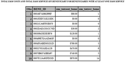
In Step 8.2, we summarize the E&M payments and services derived in Step 8.1 by beneficiary. Specifically, we use PROC SQL code to create a data set called CST.EM_COST_BENE to create two summary variables, EM_TOTCOST_BENE (which summarizes the total payments for E&M services for each beneficiary) and EM_TOTSVC_BENE (which summarizes the total count of E&M services for each beneficiary). This summarization is achieved by grouping the data by BENE_ID. Note that we label both of the variables we create, and we format the EM_TOTCOST_BENE variable to look like a dollar figure.
/* STEP 8.2: CALCULATE TOTAL E&M COSTS AND TOTAL E&M SERVICES BY BENEFICIARY */
proc sql;
create table cst.em_cost_bene as
select bene_id, sum(em_cost) as em_totcost_bene format=dollar15.2 label='TOTAL E&M COST FOR THE BENE',
sum(em_svc) as em_totsvc_bene label='TOTAL E&M SERVICES FOR THE BENE'
from em_cost
group by bene_id
order by bene_id;
quit;
Output 8.1 shows the results of Step 8.2, printing just the first 10 observations for display purposes.
Output 8.1: Total E&M Costs and Total E&M Services
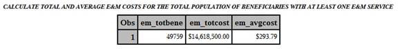
Finally, in Step 8.3, we further summarize our E&M payment and service information, but do so only for the population of beneficiaries with at least one claim for an E&M service in a physician office setting, outputting a data set called CST.EM_COST_ALL. We use PROC SQL to create a count of distinct beneficiaries called EM_TOTBENE, and a summary of total payments called EM_TOTCOST. What’s more, we perform a calculation using two of our created variables (EM_TOTBENE and EM_TOTCOST) to arrive at the average E&M payment for our population of beneficiaries with at least one E&M service, called EM_AVGCOST. We use a ‘where’ clause to ensure that our output only takes into account those beneficiaries with at least one E&M service in a physician office setting. We also label the variables we created, and format the payment and average payment calculations to look like dollar figures.
/* STEP 8.3: CALCULATE TOTAL AND AVERAGE E&M COSTS FOR ALL BENEFICIARIES WITH AT LEAST ONE E&M SERVICE */
proc sql;
create table cst.em_cost_all as
select count(distinct bene_id) as em_totbene, sum(em_totcost_bene) as em_totcost format=dollar15.2 label='TOTAL E&M COST',
(calculated em_totcost/calculated em_totbene) as em_avgcost format=dollar10.2 label='AVERAGE BENE E&M COST'
from cst.em_cost_bene
where em_totsvc_bene>0;
quit;
Output 8.2 shows the result of Step 8.3.
Output 8.2: Calculate Total and Average E&M Costs
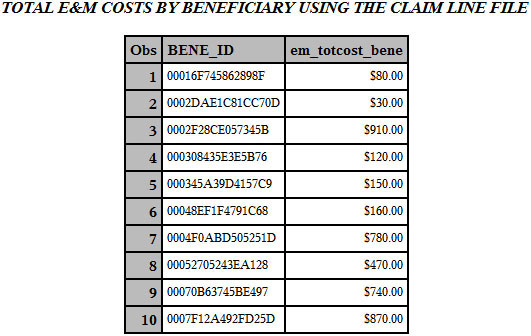
While Step 8.1 and Step 8.2 provide us with total E&M payments for each beneficiary, we can take this opportunity to arrive at the same information slightly differently. In Chapter 5, we created claim files that contained the claim header-level and claim line-level information in a single record. Can we use the line file to search for E&M codes and summarize their payments by beneficiary? Sure! In Step 8.4, we simply search the carrier claim line data for evidence of E&M procedure codes. Then, we summarize the payment on each line by beneficiary using the LINEPMT variable. Note that we could just as easily summarize the information by provider using the PRFNPI variable. Also note that we use a where clause to delimit our computation to HCPCS codes that represent an E&M service.
/* STEP 8.4: CALCULATE TOTAL E&M COSTS BY BENEFICIARY USING THE CLAIM LINE FILE */
proc sql;
create table cst.em_cost_bene_line as
select bene_id, sum(linepmt) as em_totcost_bene format=dollar15.2 label='TOTAL E&M COST FOR THE BENE'
from src.carrier2010line
where hcpcs_cd in(&emcodes)
group by bene_id
order by bene_id;
quit;
Output 8.3 shows the results of Step 8.4, printing just the first 10 observations for display purposes. Note that the output of Step 8.4 is different from the output of Step 8.2. In the Exercises section below, we ask why.
Output 8.3: Total E&M Costs by Beneficiary Using the Claim Line File
In Chapter 7, we decided to treat the claims in our inpatient claims data as stays, and we looked at stay-level summary statistics, like average length of stay (ALOS), for short-stay acute care hospitals. We will now use the total amount paid variable at the header level of the claim to calculate the total amount paid by Medicare for a stay at an acute care facility or critical access hospital. This is accomplished with slight modifications to the code we used to calculate E&M payments in Step 8.2 and Step 8.3.
In Step 8.5, we summarize total inpatient payments using the PMT_AMT variable3 in the inpatient claims data set for each beneficiary, outputting a variable called IP_TOTCOST_BENE (similar to the way we calculated total E&M payments for each beneficiary in Step 8.2). We output a data set called CST.IP_COST_BENE. Note that this PMT_AMT variable is the amount paid by Medicare to the provider for the services listed on the claim. The payment is made from the Medicare Trust Fund. Occasionally, the reader may note the presence of negative payments in the inpatient claims.4 Recall that our work in Step 7.5 in Chapter 7 excluded negative payment amounts from the inpatient claims data set.
/* STEP 8.5: CALCULATE TOTAL INPATIENT COSTS BY BENEFICIARY FOR BENEFICIARIES WITH AT LEAST ONE INPATIENT CLAIM */
proc sql;
create table cst.ip_cost_bene as
select bene_id, sum(pmt_amt) as ip_totcost_bene format=dollar15.2 label='TOTAL IP COST FOR THE BENE'
from utl.ip_2010_fnl_ss
group by bene_id;
quit;
Output 8.4 shows the results of Step 8.5, printing just the first 10 observations for display purposes.
Output 8.4: Total Inpatient Costs by Beneficiary

In Step 8.6, we use logic similar to that of Step 8.3 to summarize total inpatient payments for our population of beneficiaries with at least one inpatient claim as a whole, creating a variable called IP_TOTCOST. We also calculate average inpatient payments for this same population (IP_AVGCOST). Our output is saved to a data set called CST.IP_COST_ALL.
/* STEP 8.6: CALCULATE TOTAL AND AVERAGE INPATIENT COSTS FOR ALL BENEFICIARIES WITH AT LEAST ONE INPATIENT CLAIM */
proc sql;
create table cst.ip_cost_all as
select count(distinct bene_id) as ip_totbene, sum(ip_totcost_bene) as ip_totcost format=dollar15.2 label='TOTAL IP COST',
(calculated ip_totcost/calculated ip_totbene) as ip_avgcost format=dollar10.2 label='AVERAGE BENE IP COST'
from cst.ip_cost_bene;
quit;
Output 8.5 shows the result of Step 8.6.
Output 8.5: Total and Average Inpatient Costs for all Beneficiaries

In the above work, we have measured payments for specific services (like E&M), or in specific settings (like a physician’s office or acute short-stay hospitals). We must continue this work, using the PMT_AMT variable to summarize total Medicare Part A payments. To this end, we will summarize the total payments in each of the inpatient, SNF, home health5, and hospice data sets separately, and then as a whole. Note that we are not including the outpatient data set because, while the outpatient data set contains services performed in an institutional setting, the claims for those services are paid through Medicare Part B. Considering the fact that we are using the same PMT_AMT variable present in each data set to summarize payments, we can perform this summary of payments in a standardized fashion by utilizing a macro loop.
First, in Step 8.7, we utilize a macro loop to calculate the total Medicare amount paid by the beneficiary, which outputs a separate file for each claim type. Our macro, called CLM_LOOP, is reminiscent of the macro we utilized in Chapter 7 (Step 7.1) to delimit the data in each claim type by the beneficiaries in our enrollment data, but we added code to conditionally process inpatient data. Specifically, our CLM_LOOP macro includes a simple PROC SQL statement that should look very familiar; it is the same code we used to define other summaries of payments throughout this chapter.
There is, however, one major difference: We must figure out how to process an inpatient claims file that is named differently than the SNF, home health, and hospice files in such a way as to require special coding in the macro. Indeed, the inpatient file we are using has already been processed to exclude negative payment amounts. Therefore, the name of this file does not follow the same pattern as the other Part A files we are processing in the macro. In order to include the processing of the inpatient claims file in the macro, we use %if logic within the macro to identify the type of data set that is being processed.6 Apart from this, the code uses the claims data created in Chapter 7 (delimited by our enrollment data and, in the case of inpatient claims, type of hospital and value of payment amount), and outputs separate files for each claim type containing beneficiary identifiers (BENE_ID) and total payments associated with that beneficiary (TOTCOST_BENE). At this point, we have created payment summaries for each of the Part A claim types.
/* STEP 8.7: CALCULATE TOTAL BENEFICIARY INSTITUTIONAL COSTS USING MACRO LOOP */
%macro clm_loop(clmtyp= );
proc sql;
create table totcost_&clmtyp. as
select distinct(bene_id), sum(pmt_amt) as totcost_bene
%if &clmtyp=sn or &clmtyp=hh or &clmtyp=hs %then %do;
from utl.&clmtyp._2010_fnl
%end;
%else %if &clmtyp.=ip %then %do;
from utl.ip_2010_fnl_ss
%end;
group by bene_id;
quit;
%mend clm_loop;
%clm_loop(clmtyp=ip);
%clm_loop(clmtyp=sn);
%clm_loop(clmtyp=hh);
%clm_loop(clmtyp=hs);
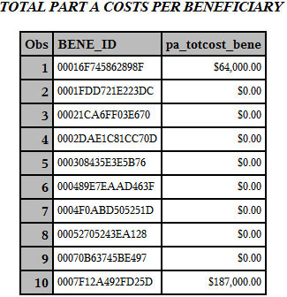
Now that we have summarized payments by claim type, we can summarize beneficiaries’ total payments for all Medicare Part A services performed during the year. To complete this task, we must sum all of the payment amounts calculated in Step 8.7 by beneficiary. Therefore, Step 8.8 utilizes the output of Step 8.7, concatenating each data set outputted from the macro used in Step 8.7. The concatenation is performed by BENE_ID so that the data set is sorted by beneficiary.7 Next, we leverage the concatenation by beneficiary to perform “by group” processing. Simply, for each beneficiary identifier (BENE_ID), we set the total Part A payment variable (PA_TOTCOST_BENE) equal to 0. Then, we add the payment summary for each beneficiary created in Step 8.7 (the variable TOTCOST_BENE) to the PA_TOTCOST_BENE variable. In this way, the PA_TOTCOST_BENE variable becomes the summary of each beneficiary’s Part A payments. When the last record for the beneficiary is reached, the final PA_TOTCOST_BENE value is outputted, and SAS processes data for the next beneficiary. The final output, called CST.PA_TOTCOST_BENE, contains one record for each beneficiary, where PA_TOTCOST_BENE represents the summation of payments from each of the institutional claim types calculated in Step 8.7.
/* STEP 8.8: SET COSTS FROM EACH CLAIMS DATA SET AND CALCULATE TOTAL INSTITUTIONAL COSTS PER BENEFICIARY */
data cst.pa_totcost_bene(keep=bene_id pa_totcost_bene);
set totcost_ip totcost_sn totcost_hh totcost_hs;
by bene_id;
if first.bene_id then pa_totcost_bene=0;
pa_totcost_bene+totcost_bene;
if last.bene_id then output;
format pa_totcost_bene dollar15.2;
label pa_totcost_bene='TOTAL PART A COSTS PER BENEFICIARY';
run;
Output 8.6 shows the results of Step 8.8, just printing the first 10 observations for display purposes.
Output 8.6: Total Part A Costs Per Beneficiary
In this chapter, we used our claims and enrollment data to program measurements of payment. Specifically, we:
• Discussed the importance of measuring payment, including the fact that reducing cost without affecting quality is a hot topic and that the measurement of utilization is linked to the measurement of cost.
• Briefly discussed the concepts of risk adjustment and price standardization.
• Programmed an algorithm to measure payments for evaluation and management (E&M) services in a physician office setting by drawing on the code we wrote in Chapter 7 to define E&M services.
• Programmed an algorithm to measure payments for acute short stay hospitals using PROC SQL and the inpatient claims data set we created in Chapter 7.
• Programmed a macro algorithm to summarize total payments by beneficiary for inpatient, skilled nursing facilities, home health agencies, and hospice claims, and included conditional processing in the macro language.
• Programmed an algorithm to calculate total Part A payments for each beneficiary by aggregating total payments from each institutional claim type for the beneficiaries in our study population.
1. Can you combine the code to identify E&M services in Chapter 7 with the code to identify E&M payments in this chapter to summarize utilization and payments in a single DATA step?
2. Can you modify the code to summarize E&M payments by provider instead of by beneficiary?
3. The output for Step 8.2 is different from that of Step 8.4. Can you explain why?
4. Can you calculate the payment by beneficiary for ambulance services?
5. How would you calculate total payments for each claim type and total Part A and Part B payments?
1 These summaries are very general, and taken from excellent information provided by MedPAC, available on MedPAC’s Medicare Background webpage at http://www.medpac.gov/payment_basics.cfm.
2 Note that we could have kept these variables in Chapter 7 and simply excluded them from our analytic file because they are not summary information.
3 For more information on the PMT_AMT variable, see the definition of Claim Payment Amount available on ResDAC’s website at http://www.resdac.org/cms-data/variables/Claim-Payment-Amount-0.
4 For more information on negative payment amounts, see the article called Negative Payment Amounts in the Medicare Claims Data, available on ResDAC’s website at http://www.resdac.org/resconnect/articles/120.
5 Technically, HHAs are paid under both Part A and Part B. Specifically, some services and supplies are paid under Part B, like visits after the hundredth visit, some drugs, and some DME supplies. For simplicity’s sake, we are assuming that all HHA expenses are paid under Part A.
6 Consider using options like mprint and mlogic to better understand the execution of this macro that contains conditional logic.
7 It is important to note that size of the data sets and efficiency may become a consideration here. One possible route around the size issue is to summarize each data set separately, and then simply sum the seven total payment amounts (one for each claim type) into a total Part A payment amount. Because the input data for this step contains one record for each beneficiary (and two variables for each of these records), it should be easy to calculate how large your data set will become.