Chapter 9: Additional Facilities in PROC X12

9.1 Model Fitting and Forecasting Using PROC X12

9.2 Seasonal Adjustment of US E-Commerce Data Using the Additional Features in PROC X12

9.3 Seasonal Adjustment of the Number of Overnight Stays

9.1 Model Fitting and Forecasting Using PROC X12

Much of the popularity of the X11 method is due to the careful correction for outliers in the series as a part of the adjustment algorithm. In this way, these outliers are prevented from affecting the calculated levels and seasonal factors, and the adjustment is more precise. In general, outliers should appear in the estimated irregular component as clear outliers, and they should not be compensated for by changing the estimated level, trend, and seasonal components. Usually, this is performed automatically, as in Section 8.2, without any intervention from the user.

In many situations, outliers are part of known phenomena, and it is possible to pinpoint them in advance to make sure that they are not overlooked. An example is a labor conflict in a transportation system that affects the quantity of sales for a period of time but that cannot affect either the seasonal factors or the level in the long run. Another example is the seasonal adjustment for monthly data for television viewing, which could possibly be different in years with Olympic Games, usually in July or August. These are examples of so-called additive outliers that influence just a single or a few observations. Other types of outliers are due to level shifts that lead to a permanent shift in the series level. An obvious example is the opening of a new production facility that increases sales on a permanent basis. In PROC X12, you can specify such outliers, which are then treated by dummy variables. Another possibility is to start automatic outlier detection, which ends up with a list of potential outliers. Then you can correct the values if the outliers are due to errors or identify them as outliers before the usual seasonal adjustment algorithm.

PROC X12 also includes methods for correcting calendar effects. For example, you can correct series for retail sales for the number of trading days in each month. This idea is extended further by correcting for numbers of Mondays, the number of Tuesdays, and so on, for each month. This is important for series with a clear weekly pattern, such as the numbers of theater tickets sold. These features correct for the fact that the seven-day week is out of phase with the number of days in a month and also for the fact that the months are of different lengths. The effect of leap years is treated in a similar way.

Another type of modification is corrections for calendar effects caused by holidays, such as Easter. This is especially important in the case of Easter, because it can fall either in the first or second quarter of the year. Special predetermined corrections have special reference to the American market in cases such as Independence Day, which affect series differently if it falls on a Sunday or on a trading day.

Special days in local non-US calendars can also be included in the seasonal adjustment, using features for correction of known external events mainly introduced for outliers.

The X11-ARIMA method is also included among the features of PROC X12. It improves the seasonal adjustment of the latest observation by forecasting the time series so that the symmetric moving average that defines the estimated trend-cyclic component can be applied. The forecasts are generated by fitting seasonal ARIMA models (also known as Box-Jenkins models; see Box and Jenkins [1976]) as introduced in Section 7.5. You can provide the exact specification of the model type, but PROC X12 also offers methods for automatically selecting a suitable ARIMA model. In fact, PROC X12 can be used for the automatic prediction of time series as an alternative to PROC ESM, which was applied in Chapter 6 for seasonal time series. PROC X12 also derives forecasts in a way similar to PROC VARMAX, which was introduced as a more model-based procedure in Chapter 7.

9.2 Seasonal Adjustment of US E-Commerce Data Using the Additional Features in PROC X12

In this section, the time series of US e-commerce is seasonally adjusted in various ways, including the refinements offered by PROC X12 as an extension of the basic seasonal adjustment by the X11 method in Section 8.2.

In the first application, PROC X12 is used to obtain a seasonal adjustment in the multiplicative version, which is applied as a trend seen to dominate the series (see Program 9.1). The pre-modeling features of PROC X12 fit a linear regression model to the relevant series. But as the seasonal adjustment is done by the multiplicative method, the linear model has to be fitted to the logarithmically transformed series. That series corresponds to a multiplicative model for the original series, and fitting the linear model to it is done by the TRANSFORM statement. The TRANSFORM statement can also be used for more advanced transformations such Box-Cox transformations in order to prevent heteroscedasticity.

Program 9.1 Exploiting the additional features of PROC X12

PROC X12 data=sasts.E_commerce date=date;
var E_commerce;
transform function=log;
automdl ;
regression predefined=(td);
outlier;
forecast lead=7 ;
ods output ForecastCL=predicted;
x11;
output out=out a1 d10 d11 d12 d13;
run;

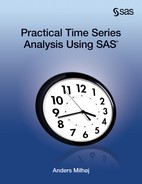
The REGRESSION statement gives an adjustment for weekdays because the trading day correction (the td option for the predetermined independent variables) provides dummy variables for Mondays, Tuesdays, and so on. If, for example, the sales are highest on Mondays, the series is adjusted for the fact that the number of Mondays in a quarter varies depending on the calendar. The estimated coefficients of these dummies are printed in text output; see Output 9.1. Many of these estimates are just significant at a 5% test level but their influence is low because the largest impact is the reduction of 2% by the number of Saturdays. Intuitively, the effect should be small for quarterly data because the number of, say, Saturdays in a quarter is almost constant. The portmanteau test for a simultaneous effect for all days of the week, however, shows significance; see Output 9.2.

Output 9.1 Estimated parameters

Output 9.2 Portmanteau test statistic

The outlier statement provides a more formal testing for outliers in the observed series than the automatic modification of their effect provided in the ordinary X11 adjustment process. The critical value for the outlier test is printed in the output. It depends on the number of observations and in this example of 42 observations, it has the value 3.59; see Output 9.3.

Output 9.3 Critical values for outlier tests

Just a single observation is identified as an observation with a significant value of the irregular component, which in the output is denoted as an additive outlier. The coefficient is negative and the value – 0.13 corresponds to about a roughly 13% lower level of e-commerce than had been expected. This is the 1994Q4 value, which is in the very beginning of the observed series. It is therefore possible that this outcome is due to the fact that the volume of e-commerce up to Christmas had not reached a stable level. Moreover, one level shift is detected, 2003Q3, where the level of the series seems to have increased permanently by around 11%.

The observed series is then corrected based on these outliers and on deterministic calendar effects before the usual X11 method is applied. The series is extended by forecasts following the lines of the X11-ARIMA method.

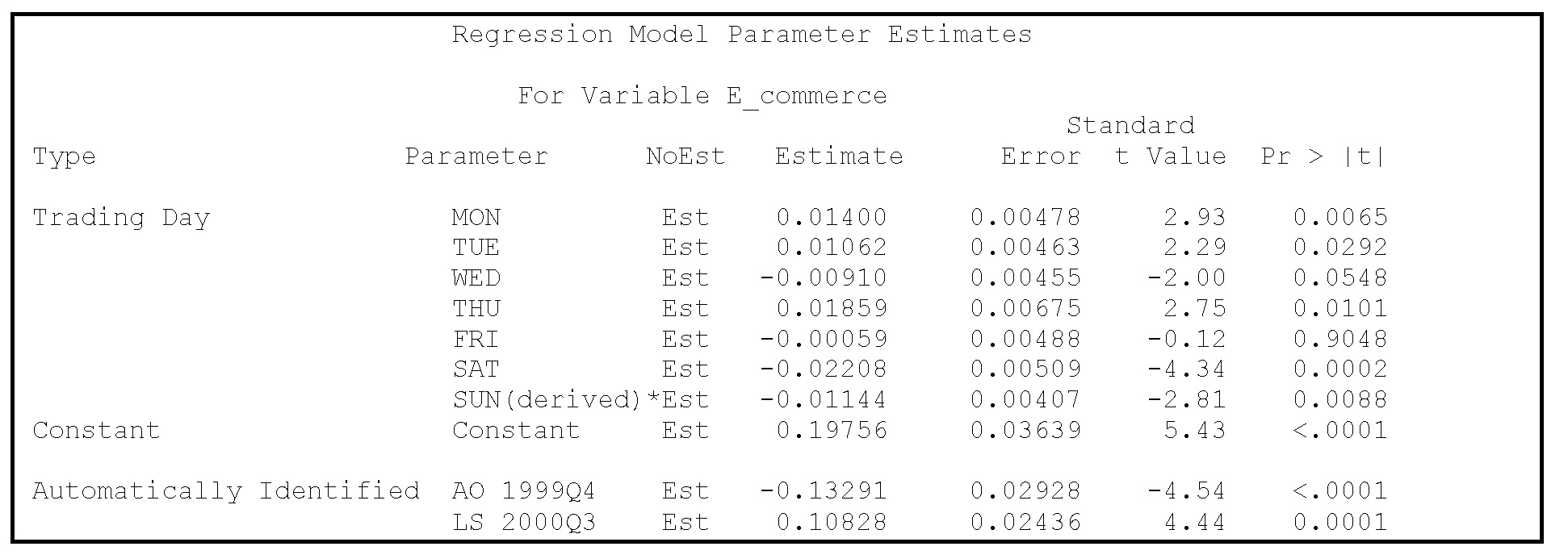
The AUTOMDL statement gives an automatic identification of a time series model used for forecasting purposes and provides an improvement of the adjustments of the latest observations. An exact model is not specified; the best model is found among a battery of usual standard models. The listed output shows that the chosen model in this example is the ARIMA(2,0,0)×ARIMA4(0,1,1) model:

This is a Box-Jenkins seasonal ARIMA model; see Section 7.5. The parameters are estimated in Output 9.4.

Output 9.4 Estimated ARIMA parameters

You can specify a particular Box-Jenkins model using an ARIMA statement. The useful airline model for quarterly data, the ARIMA(0,1,1)×ARIMA4(0,1,1) model

is, for example, specified by substituting the AUTOMDL statement with the following ARIMA statement:

arima model=((0,1,1)(0,1,1)4);

Often this model is preferred even if some particular model gives a better fit for a particular series. To this end, the option acceptdefault in the AUTOMDL statement is employed:

automdl acceptdefault;

By this option, the airline model is accepted except for series where the model gives an unacceptable fit when judged by the standard Ljung-Box test. See, for example, Box and Jenkins (1976).

The most important series are stored in an output data set by the OUTPUT statement, and then they are plotted by PROC SGPLOT. The adjusted series behaves like a smooth curve even if, by definition, it includes the irregular component. (See Figure 9.1.) The irregular component is dominated by the outlier for the first observation, which is 13% less than expected and corresponds to the factor 0.87 on the plot. (See Figure 9.2.)

Figure 9.1 Adjusted series of US e-commerce compared to original series

Figure 9.2 Irregular component for US e-commerce

The forecasts constructed by PROC X12 are plotted in Figure 9.3. They are calculated using the fitted ARIMA model. They are printed in the text output, and this table is stored as a SAS data set named Predicted by the ODS OUTPUT statement. Note that this data set is created by the code in Program 9.1 and is not a part of an OUTPUT statement or output option in the ordinary X12 syntax. This data set is amended in Program 9.2 to the observation data set, and these forecasts and data for the latest years in the data set are then plotted using PROC SGPLOT. However, the data set named Predicted contains both the original series and the log-transformed series. Only the predicted values of the original series should be amended to the original series. Because the log-transformed values are close to 1, the where=(forecast>100) option in the SET statement ensures that only forecasts of the original values are selected, because they are all above 100.

Program 9.2 Plotting the predictions obtained using PROC X12

data plot;
set sasts.Ecommerce predicted(where=(forecast>100));
run;
PROC SGPLOT data=plot;
series x=date y=Ecommerce/markers;
series x=date y= forecast/markers ;
series x=date y=lowerCL/lineattrs=(pattern=solid color=black);
series x=date y=upperCL/lineattrs=(pattern=solid color=black);
run;

Figure 9.3 Forecasts of US e-commerce

The forecasts basically have the form of an upward trend with some seasonal structure. Due to the multiplicativity of the model, the seasonal deviations increase as the level increases. Of course, the plotted 95% confidence limits also broaden as the level increases and also as the uncertainty increases for large forecasting horizons.

9.3 Seasonal Adjustment of the Number of Overnight Stays

In this section, the time series of the number of overnight stays by US citizens at Danish hotels is seasonally adjusted in various ways, including with the refinements offered by PROC X12. The forecasting of this series was considered in Chapter 6. This monthly time series shows a clear seasonal pattern, having high values in the summer months, but in the winter months the number of US citizens spending nights at Danish hotels is rather low (they are probably mainly business travelers). (See Figure 9.4.) The series is observed from January 1992 to May 2010, giving a total of 221 observations.

Figure 9.4 Number of overnight stays by US citizens in Denmark

PROC X12 is used in Program 9.3 to obtain a seasonal adjustment in the additive version with the option mode=add in the X11 statement, which is applied because no trend is seen to dominate the series. Moreover, only additive outliers are searched for because no level shifts are seen in Figure 9.4. This is made possible by the option type=ao in the OUTLIER statement.

Program 9.3 Code for PROC X12 for the series of number of overnight stays at Danish hotels

proc X12 data=sasts.hotel date=date;
var number_of_nights;
outlier type=ao;
x11 mode=add force=totals;
regression predefined=(td easter(1));
automdl;
forecast lead=24;
ods output ForecastCL=predicted;
output out=Figur9__5out a1 d10 d11 d12 d13 d11f;
run;

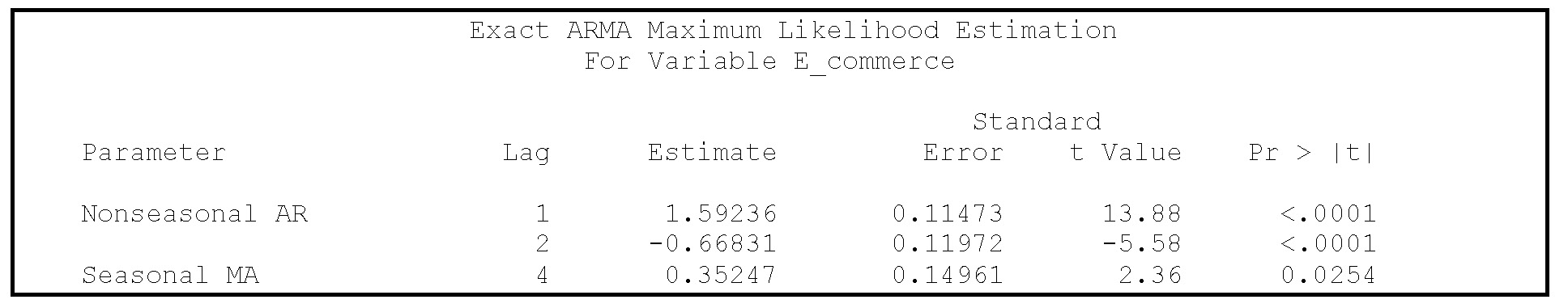
The REGRESSION statement gives an adjustment for weekdays and for the Easter season using predefined explanatory variables stated in parentheses for the predefined option. The trading day correction (the td option for the predetermined independent variables) provides dummy variables for Mondays, Tuesdays, and so on. If, for example, the number of stays is highest on Fridays, the series is adjusted for the fact that the number of Fridays in a month is either four or five depending on the calendar. The estimated coefficients of these dummies are printed in the text output (Output 9.5), but only the negative effect caused by the number of Mondays is clearly significant; the others are hardly significant when considered individually. The portmanteau test for a simultaneous effect for all days of the week, however, shows significance; see Output 9.6. The leap year correction is insignificant.

Output 9.5 Parameter estimates

Output 9.6 Portmanteau tests

The Easter holiday is specified only as a dummy for whether Easter Sunday falls in March or April, but it is possible to specify the effect of Easter more flexibly according to the nature of the series. In the easter option, a number in parenthesis indicates dummy variables for these days so that easter(3) gives a correction for whether Easter Friday, Saturday, and Sunday are in March or April. You can specify more than one easter option, which would result in a very flexible correction for a scenario with high activity on the trading days before Easter and extraordinary low activity during the Easter holidays. In this example, the Easter effect is significant at a 5% test level, resulting in a reduction of the number of overnight stays during the month that includes Easter Sunday.

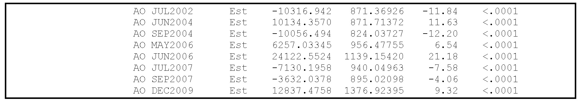
The OUTLIER statement provides a more formal testing for outliers in the observed series than the automatic modification of their effect provided in the ordinary X11 adjustment process. The critical value for the outlier test is printed in the output and depends on the number of observations; in this example of 221 observations, it has the value 3.98. Even if this critical value is high, the number of identified outliers is very large; see Output 9.7. Several observations are identified as observations with a significant value for the irregular component, which in the output is denoted as an additive outlier.

Output 9.7 Regression parameters

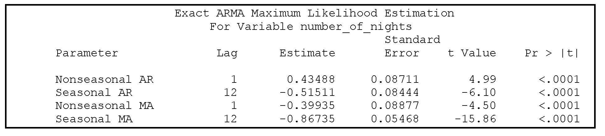
The AUTOMDL statement automatically identifies a time series model used for forecasting purposes, which is an improvement on the adjustments of the latest observations. Because no exact model is specified, the best model is found among the usual standard models. In the listed output, the chosen model in this example is the ARIMA(1,0,1)×ARIMA12(1,1,1) model:

This model is a Box-Jenkins seasonal ARIMA model. (See Section 7.5.) The parameters are estimated in Output 9.8. The model is found by automatic criteria but which model is actually selected is of minor importance. Many seasonal ARIMA models fit the series well enough to provide the basis for the forecasting of future observations to be used in the seasonal adjustment algorithm, and the precise form of the fitted model is of no interest.

Output 9.8 Estimated ARIMA parameters

In this example, you might want the yearly total number of overnight stays in the adjusted series to equal the actual observed yearly number of overnight stays. This is obtained by the option force=totals in the X11 statement:

x11 mode=add force=totals;

In Program 9.3, these corrections are stored in the output data set as the D11F series. Figure 9.5 shows the adjustment factors used to do the corrections. The order of these corrections is at most 100, which is small compared with the minimum value around 20000 of the observed series.

Figure 9.5 Adjustments in order to obtain correct yearly totals

The most important series are stored in an output data set by the OUTPUT statement, and then they are plotted by PROC SGPLOT. In the output data set, all series are named as number_of_nights, which is the name of the original series, followed by an underscore and the name of the series. For this example, the final adjusted series is named number_of_nights_d11.

Figure 9.6 presents the plot of the estimated trend-cyclic component obtained by using PROC X12. This seasonal adjustment is a bit unsatisfactory because the fitted trend seems very volatile. In the printed output (along with the table of the estimated trend-cyclic component, the D12 series), it is stated that this trend cycle is calculated by a “13 term Henderson moving average.” One possible remedy is to increase the length of the moving average in this formula in order to obtain a smoother trend curve. In the call of PROC X12 this is done in the X11 statement with a trendma option. A moving average with a length of 23 is obtained by:

x11 mode=add trendma=23;

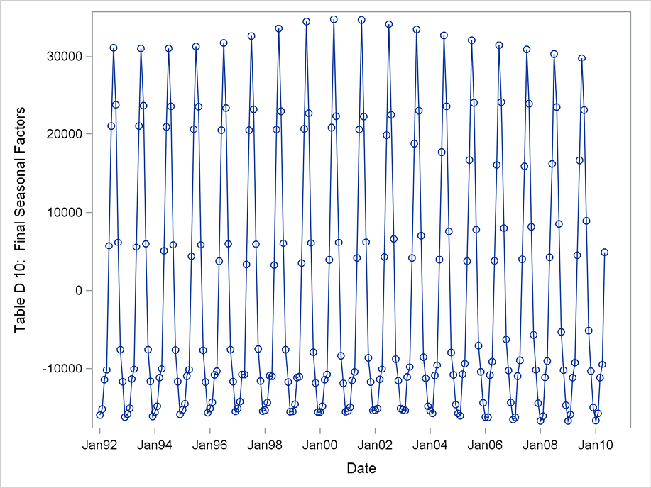
This results in a more realistic smooth trend. (See Figure 9.7.) Moreover, the adjusted series also behave more smoothly even if the adjusted series by definition includes the irregular component. (See Figure 9.8.) As stated above, many extreme values exist for the irregular component, and they are clearly seen in Figure 9.9, especially the May 2006 value of about 23000. This must be due to something special such as a large conference with many American participants. The seasonal component, shown in Figure 9.10, is rather static, with the highest value in July. A closer look reveals that the June value has declined from around 20000 to 16000 overnight stays during the observed 18 years.

Figure 9.6 Trend-cyclic component using default smoothing

Figure 9.7 Trend-cyclic component using a longer order of the smoothing average

Figure 9.8 Seasonal adjusted values of the number of overnight stays compared with the original series

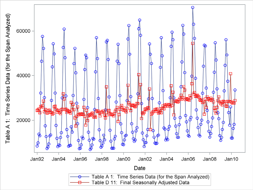
Figure 9.9 Irregular component for number of overnight stays

Figure 9.10 Seasonal component for number of overnight stays

The forecasts constructed by PROC X12 are calculated using the fitted ARIMA model. They are stored as a SAS data set named Predicted specified in the OUTPUT statement in this application of PROC X12. This data set is amended to the observation data set. These forecasts and data for the latest years in the data set are then plotted using PROC SGPLOT. See the code in Program 9.4. The plot of the predictions with confidence limits is shown in Figure 9.11. In SAS version 9.3 with the ETS 12.1 update, this plot is found in the standard output but the series plots for Figure 9.5–Figure 9.10 are not produced automatically.

Program 9.4 Plotting predictions derived by PROC X12 for the number of overnight stays

data plot;
set sasts.hotel predicted;
run;
PROC SGPLOT data=plot;
series x=date y=number_of_nights/markers;
series x=date y= forecast/markers ;
series x=date y=lowerCL/lineattrs=(pattern=solid color=black);
series x=date y=upperCL/lineattrs=(pattern=solid color=black);
where date>’31dec2006’d;
run;

Figure 9.11 Forecasts of number of overnight stays

The forecasts look like a very probable continuation of the observed time series. The forecasts’ limits seem to be very narrow due to the rather precise estimate of seasonality in the series. Moreover, the series having no trend in the observation period is forecast to be rather static, leading to a high expected precision. These forecasts are of the same quality as the forecasts calculated in Section 6.4 with the dedicated forecasting procedure PROC ESM. In practice, however, these forecasts are more a by-product of the seasonal adjustment. It is doubtful whether any user will turn to a seasonal adjustment procedure in order to forecast a time series.