Chapter 3: Aggregation Using PROC TIMESERIES
3.1 Aggregation
Observations of continuous series are usually sampled at distinct points in time, leading to discrete equidistant time series. For example, you could record the outdoor temperature at all integer hours. But a series in continuous time could (at least in theory) be observed by some analog recording device, perhaps as a curve drawn on a piece paper. Such a curve could easily be digitalized and converted to a series in discrete time with very short time intervals, such as milliseconds. Modern technical measurement devices produce such curves on the basis of very frequent discrete observations. Such original data sources already have, in reality, the form of a discrete equidistant time series observed with a very high frequency. High-frequency data series can, however, be inconvenient for further analyses if you are interested in long-term aspects and the numbers need to be aggregated to more relevant time intervals.
You can perform these aggregations in many ways based on the current interest of the analysis and the nature of the time series. You could aggregate the outdoor temperature by using just point-in-time measurements such as every integer hour. However, an average of many observed temperatures during a full hour might also be relevant. You might also be interested in other possibilities, such as the maximum or minimum temperature, or even a number for the standard deviation of observations within an hour.
Other time series are constructed from transactional data. One simple example is a series of total sales within a month, which by definition is the sum of every single sale. In modern computer systems, these sales are recorded as a point in time specified precisely at the level of seconds. Also included is information about the type of good being sold and the corresponding amount of money. In order to analyze such data by the methods in this book, these numbers have to be converted into series of, say, monthly sales.
Within the SAS system, this aggregation is performed by PROC TIMESERIES, as illustrated in this chapter. You could also perform the aggregation along with the analyses. For example, PROC ESM, which is used for forecasting by exponential smoothing methods in Part 2, includes statements and options for aggregation as an integrated part of the procedure call.
3.2 PROC TIMESERIES
As an example of an irregularly observed time series, a series of recordings of a counter at a photocopying machine is used. Every time a technician is called to the machine for repair or service, he records the counter, but because he arrives at irregular intervals, these recordings form a messy time series. The observed series is shown in Figure 3.1.
Figure 3.1 Observations of the counter position of a copy machine
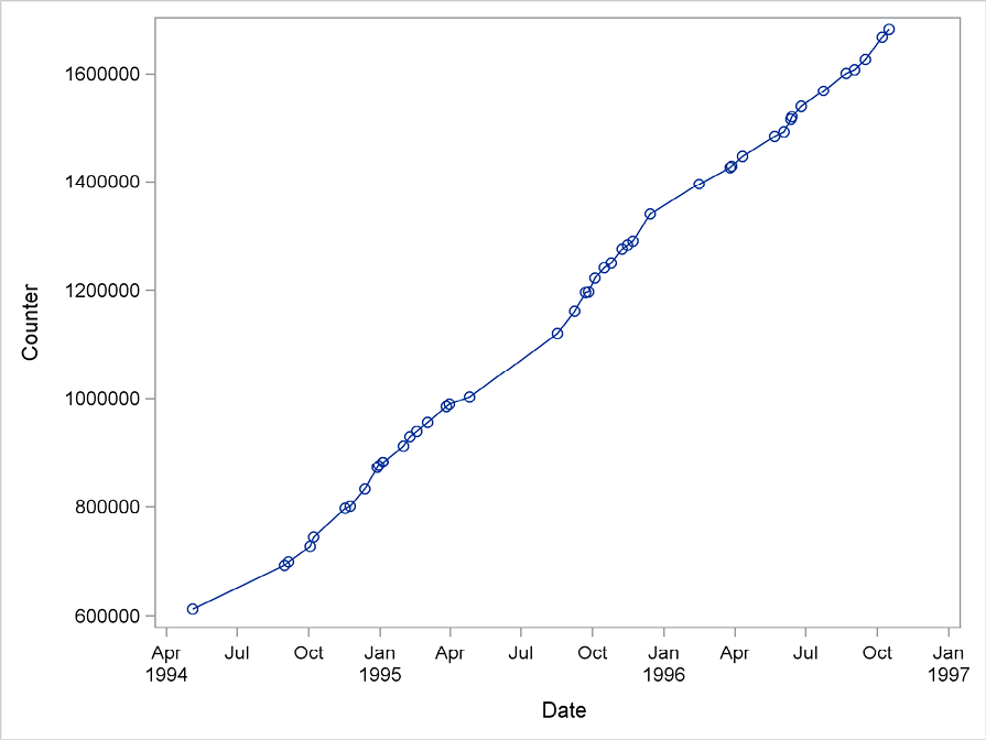
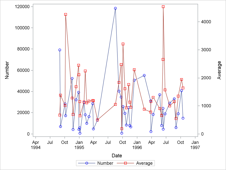
The actual number of copies made by the photocopy machine during the time interval between two visits of the service technician is calculated as the difference of the counter position between the two consecutive visits. In Program 3.1, the SAS function dif in the DATA step calculates a new variable for the number of days and also the number of copies made between two visits. The number of copies is plotted by PROC SGPLOT in Figure 3.2, along with the average number of copies between two visits. Such plots could also be drawn by PROC TIMESERIES, but because the purpose of this application of the procedure is to derive output series for further analyses by other SAS procedures, the plot is drawn by a separate procedure call outside PROC TIMESERIES.
Program 3.1 Code generating the number of copies between two service visits
data a;
set sasts.copy_machine;;
number=dif(counter);
days=dif(date);
average_number=number/days;
run;
PROC SGPLOT data=a;
series x=date y=number/markers;
series x=date y=average_number/markers y2axis;
run;
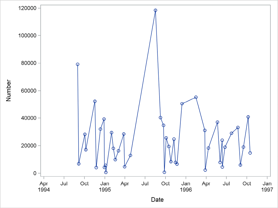
Figure 3.2 Plot of the number of copies
The two time series plotted in Figure 3.2 are not equidistant, so in order to apply most of the facilities for time series analysis, they have to be aggregated. The application of PROC TIMESERIES in Program 3.2 aggregates the series to monthly totals, which are then plotted by PROC SGPLOT; see Figure 3.3.
Program 3.2 A first application of PROC TIMESERIES
PROC TIMESERIES data=a out=b;
id date interval=month accumulate=total setmissing=missing;
var number;
run;
PROC SGPLOT data=a;
series x=date y=number/markers;
run;
The time index, the variable date, is given in the mandatory id statement, which also contains the relevant information for the type of aggregation required for the analyses. The option setmissing=missing specifies that months without any observations should be regarded as missing values, which in this situation means not existing. The aggregated series then contains a gap for months such as May to July 1995 where no observations are plotted. Among the other possibilities for missing observations is setmissing=average, which replaces missing observations by the overall average for all observations, and setmissing=previous or setmissing=next, which replaces the missing observation with the previous or next available observed value. For series of stock market quotations, the option setmissing=previous is standard practice.
Figure 3.3 Number of copies aggregated to monthly totals by PROC TIMESERIES
This aggregation by totals might not be what you want in this situation, because a large number results if the copy machine has not been maintained for a long time. This makes all copies over many months appear in a single month. This result might be useful when the user of the machine is charged for the number of copies after each visit by the service man, but not in months with no visits. But if the actual use of the copy machine is of interest, more care has to be taken, and the best method is to interpolate the missing monthly number of copies. This is preferably done by the interpolation procedure PROC EXPAND. See Section 4.2 in the next chapter, where this example about the copy machine is continued.