Chapter 7: Exponential Smoothing versus Parameterized Models
7.1 Exponential Smoothing Expressed as Autoregressions
7.3 Fitting Autoregressive Models
7.6 Estimating Box-Jenkins ARIMA Models in SAS
7.7 Forecasting Fertility Using Fitted ARMA Models in PROC VARMAX
7.8 Forecasting the Swiss Business Indicator with PROC ESM
7.9 Fitting Models for the Swiss Business Indicator Using PROC VARMAX
7.1 Exponential Smoothing Expressed as Autoregressions
Forecasts using exponential smoothing are constructed by a very simple algorithm. In fact, these forecasts could easily be calculated by hand before computers were available. Often, experience shows that the forecasting performance of exponential smoothing procedures is as good as the performance of more refined and complicated methods. Therefore, they are still frequently used.
The exponential smoothing procedures define the predictions as the weighted averages of previous observations, which tend to give the most weight to the most recent observation. Even if an exact formula of this kind does not exist in all situations, the forecasts are, in practice, closely approximated by such weighted averages.
For example, simple exponential smoothing defines the smoothed value recursively by:
![]()
This is easily iterated to

because the initialization is ![]() . Note that the weight coefficients add up to 1, which defines the smoothed component as a true weighted average of the present and past observations.
. Note that the weight coefficients add up to 1, which defines the smoothed component as a true weighted average of the present and past observations.
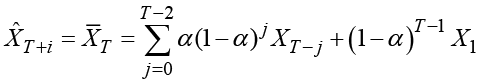
The estimated value ![]() of the level for the last observation (which is used as predictions for all horizons i) is written as an explicit average of the values of the time series in the observation period as
of the level for the last observation (which is used as predictions for all horizons i) is written as an explicit average of the values of the time series in the observation period as
 .
.
The forecasts for most other exponential smoothing methods are written in the same form, which can generally be formulated as

where the coefficients Πj add up to 1. These coefficients are exponentially decaying functions of the smoothing parameter α (and also of ω in the case of seasonal exponential smoothing). This is the explanation for naming all these methods “exponential smoothing.”
Exponential smoothing is a variant of fitting autoregressive time series models to data. Some of these models are discussed in the following sections.
7.2 Autoregressive Models
The autoregressive model of order p, denoted AR(p) has the form
 .
.
The parameter µ is the mean of the series, but it could be replaced by a linear function of the time index in order to incorporate a trend in the model. The remainder terms ![]() form a series of independent random variables with the expected value of 0. Series of this form are also called white noise series. This model describes series for which past values of the series itself include information about the future value of the series.
form a series of independent random variables with the expected value of 0. Series of this form are also called white noise series. This model describes series for which past values of the series itself include information about the future value of the series.
The forecasts in the AR(p) model are derived recursively for horizons i = 1, 2 ,3 ... by

where actual observed values ![]() are of course used for i ≤ j.
are of course used for i ≤ j.
Parameter values ![]() apply to series in which deviations from the mean value are of the same sign for many periods. In regression analysis, this is often denoted as positive autocorrelation. A simple example is sales of ice cream. Sales might be higher than expected during periods of hot weather and lower than expected during periods of cold weather. This behavior is in conflict with standard assumptions of independence among the remainder terms, and it is often seen as a model shortcoming in statistical models where some important explanatory variable is missing (such as the outdoor temperature in the ice cream example).
apply to series in which deviations from the mean value are of the same sign for many periods. In regression analysis, this is often denoted as positive autocorrelation. A simple example is sales of ice cream. Sales might be higher than expected during periods of hot weather and lower than expected during periods of cold weather. This behavior is in conflict with standard assumptions of independence among the remainder terms, and it is often seen as a model shortcoming in statistical models where some important explanatory variable is missing (such as the outdoor temperature in the ice cream example).
Parameter values ![]() describe series with a jagged behavior as positive deviations from the mean that are followed by negative deviations from the mean. In a sales series, a conflict in the labor market might reduce the sales one month but only postpone them to the next month. As a result, total sales over the two months remain constant.
describe series with a jagged behavior as positive deviations from the mean that are followed by negative deviations from the mean. In a sales series, a conflict in the labor market might reduce the sales one month but only postpone them to the next month. As a result, total sales over the two months remain constant.
In fact, many possible outcomes, such as business cycles, could be generated by this definition of autoregressive models. The data example in Section 7.9 shows only a few of these possibilities. A more thorough theoretical exposition is outside the scope of this book. The main point here is that the fitting of such parameterized models is a first step in building real statistical, econometric models for the series.
The formulation of autoregressive models described above corresponds to a situation for which a mean value of the series is assumed to exist. Therefore, these models are of no use for series with shifting levels, such as many stock market series. In those situations, it is often possible to consider the series of first-order differences ![]() as having a constant mean. If the series is dominated by a linear trend, the first-order differences vary around the slope parameter, and again the series of differences has a constant mean value.
as having a constant mean. If the series is dominated by a linear trend, the first-order differences vary around the slope parameter, and again the series of differences has a constant mean value.
Autoregressive models could be formulated for the differenced series. The technique could even be generalized further, such as by differencing the differenced series once more, or by applying seasonal differences as described in Section 7.5. As a result, you end up with very successful models. In this way, autoregressive modeling has a huge range of applications.
7.3 Fitting Autoregressive Models
The parameters ![]() and
and ![]() can be estimated by a minimization of the sum of squared residuals
can be estimated by a minimization of the sum of squared residuals
 .
.
The value of p should be at least 12 or preferably 13 for monthly data in order to allow for seasonality.
The drawback of this procedure is that the parameters are estimated with some uncertainty because the number of parameters might be fairly large compared with the number of observations. However, many of the autoregressive parameters ![]() are often insignificant, and taking this into account reduces the estimation burden. It is possible to test for estimated autoregressive parameters
are often insignificant, and taking this into account reduces the estimation burden. It is possible to test for estimated autoregressive parameters ![]() being 0. In this way, you could determine the value of the lag number p by applying statistical testing.
being 0. In this way, you could determine the value of the lag number p by applying statistical testing.
Another possibility is to apply some automatic criteria for best fit and derive an optimal model. Such criteria include a premium for a small error variance, but because every parameter reduces the residual sum of squares, simply minimizing the sum of squares results in too many parameters. To avoid having too many parameters, a “penalty” for extra parameters is added to the criterion.
Frequently used criteria are the Akaike information criterion (AIC) and Schwarz’s Bayesian Criterion (SBC). These criteria are for the length of the observed time series (represented by T), the number of observations used in the estimation, and the order of the fitted autoregressive model (represented by p) defined as

and
 .
.
In most practical situations, the penalty term (the first term) is more severe for SBC than for AIC as ![]() for all time series. Forecasting by automatically finding an order p of an AR(p) model and then predicting using the estimated parameters is referred to as STEPwise AutoRegression (STEPAR).
for all time series. Forecasting by automatically finding an order p of an AR(p) model and then predicting using the estimated parameters is referred to as STEPwise AutoRegression (STEPAR).
This procedure could be refined and extended in many directions. It can be seen as a starting point of a statistical model-building process for the time series and not an easy-to-use black box procedure. A classical reference to parameterized time series analysis is Box and Jenkins (1972).
7.4 Autocorrelations
Violations of the independence assumption can be considered as a simple plot of the forecast errors in the observation period. The autocorrelation function is briefly introduced in this section for two purposes. First, the autocorrelations for the series of forecast errors form a basis for investigating whether the errors behave in a systematic way, which indicates that the forecasting method is inadequate. Second, the autocorrelation function of an observed time series can be used to study its behavior and to identify a proper statistical model to the series.
The kth-order autocorrelation is defined as the correlation between values of the time series with a time lag of k periods. In order to theoretically validate such a definition, the series is supposed to be stationary so that the correlation coefficients depend not on the timing but only on the time lag k. For an observed time series, this autocorrelation is estimated by
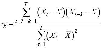
where ![]() denotes the average of the observed series. This empirical autocorrelation can be calculated even if a theoretical autocorrelation is meaningless. These estimated autocorrelations define a method for fitting ARIMA models in the Box and Jenkins (1972) procedure for fitting ARIMA models to an observed time series.
denotes the average of the observed series. This empirical autocorrelation can be calculated even if a theoretical autocorrelation is meaningless. These estimated autocorrelations define a method for fitting ARIMA models in the Box and Jenkins (1972) procedure for fitting ARIMA models to an observed time series.
The calculated autocorrelations for the series of forecasting errors are often applied to validating the forecasting procedure. If some dependency is present in the forecast errors, this dependency can be exploited in order to improve the forecasts, because the dependencies are seen as autocorrelations significantly different from zero. For the forecast errors, it is important to determine whether these autocorrelations are close to zero. You can do this graphically by simply looking at a plot of the autocorrelations. More explicit testing procedures rely on the result that the variance of the autocorrelations is at most T-1, but more precise formulas exist. Another possibility is to define a test statistic as the sum of squares of the calculated autocorrelations, which could be used as a chi-square test statistic. In the example in Section 7.8, the autocorrelation function is applied in the validation of the forecasting method, but more advanced testing is beyond the scope of this book. For more information about time series within a SAS framework, see Brocklebank and Dickey (2003).
7.5 ARIMA Models
All moving average representations of the exponential smoothing methods discussed in Section 5.6 are series in terms of past forecast errors. These representations are in the form

but include only a finite number of terms in the summation, corresponding to the length of the observed time series. The term ![]() is considered a series of independent, identically distributed remainder terms with a mean of 0. In the situation where only a finite number of terms, such as q, are included in the sum, the model is denoted MA(q). This model is often written in the form
is considered a series of independent, identically distributed remainder terms with a mean of 0. In the situation where only a finite number of terms, such as q, are included in the sum, the model is denoted MA(q). This model is often written in the form
![]()
where the parameter ![]() is the mean value. The remainder term, the prediction error
is the mean value. The remainder term, the prediction error ![]() , can be considered as the unexpected part of the observation
, can be considered as the unexpected part of the observation ![]() . This can be used in intuitive interpretations of the moving average models because past values of these remainder terms could easily affect future values of the time series.
. This can be used in intuitive interpretations of the moving average models because past values of these remainder terms could easily affect future values of the time series.
Similar to autoregressive models, moving average models can be applied to a time series after a differencing. When a MA(1) model is fitted to the series of first-order differences, the resulting model has a clear interpretation. If the change from time –t–2 to time t–1was unexpectedly high (meaning that ![]() was positive due to a positive error term
was positive due to a positive error term ![]() ), then you expect that the difference
), then you expect that the difference ![]() will be negative as predicted by the term
will be negative as predicted by the term ![]() (assuming
(assuming ![]() is positive). This is often the situation if the observed series is some type of activity that has to take place but for which the timing is not fixed. An agricultural example is the number of pigs that are slaughtered. This number might vary from month to month, but because every animal has to be slaughtered, a high number one month leaves fewer animals to be slaughtered next month.
is positive). This is often the situation if the observed series is some type of activity that has to take place but for which the timing is not fixed. An agricultural example is the number of pigs that are slaughtered. This number might vary from month to month, but because every animal has to be slaughtered, a high number one month leaves fewer animals to be slaughtered next month.
It turns out that simple exponential smoothing can be expressed as a MA(1) model with parameter ![]() for the series of first-order differences. This is because the expression
for the series of first-order differences. This is because the expression
![]()
or equivalently
![]()
applied recursively becomes the expression

This expression is similar to the expansion obtained for simple exponential smoothing in Section 5.6.
Similarly, double exponential smoothing can be interpreted as a moving average model of order two applied to the series of second-order differences, which is the series of differences of the series of differences.
The class of moving average models can be combined with seasonal components to create more elaborate models with a wide range of applications for series that show seasonality. A model that is often applied to seasonal time series is the so-called Airline Model, which was famously applied to a time series of airline passengers by Box and Jenkins (1972). The Airline Model is often referred to in SAS documentation. It has a multiplicative form, including both a seasonal and an ordinary differencing, which is expressed as a polynomial in the backward shift operator. Remember that the backshift operator B is defined by
![]()
![]()
The model is really formulated as a model for the series with a multiplicative differencing structure that is obtained by taking seasonal differences of first-order differences. The moving average part has basically the same form:

The model as a model for the original series ![]() is often written as:
is often written as:

This clearly explains why the model is named a multiplicative seasonal moving average model. This model is applied in Chapter 9 to seasonal adjustments by more advanced methods.
A further generalization is the combination of autoregressive and moving average models that allows for very general autocorrelation structures. The basic form of these models is the ARMA(1,1) model:
![]()
The mean value in this notation is

More terms can be added to both the autoregressive and the moving average part. More terms would lead to the general model denoted as ARMA(p,q). If a differencing is also applied, the class of models is denoted ARIMA(p,d,q), where d is the number of differences applied, usually d = 0 or d = 1. If seasonal factors are present, the model is denoted ARIMA(p,d,q) × ARIMAS(P,D,Q), when you assume that the seasonal cycle is S periods. The airline model is written as ARIMA(0,1,1) × ARIMA12(0,1,1). See Box and Jenkins (1972) and Brocklebank and Dickey (2003) for more information.
When forecasting a moving average series, the future error terms are unknown, and they are predicted as their expected value 0 while past forecast errors are assumed to be known. The forecasts in a MA(q) process therefore equal the mean value of the series for horizons i > q. The prediction variance in a MA(q) model increases to the upper limit
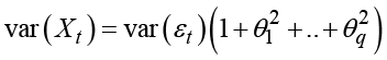
and the confidence limits are stable, increasing to an upper limit and not exploding as in many of the applications in Chapter 5.
If the order of the moving average model is infinite, the forecasts are non-constant and the prediction variance is an increasing function of the forecast horizon:

This sum could converge to a finite limit. But in all models that include a trend or a difference operation, it tends to infinity. Often, the moving average representation of all exponential smoothing procedures also increases to infinity at a very fast rate.
7.6 Estimating Box-Jenkins ARIMA Models in SAS
The models proposed by Box and Jenkins (1972), the seasonal ARIMA models, are fully specified statistical models for which it is possible to establish the likelihood function and maximum likelihood estimation. Likelihood ratio testing is then performed using numerical methods because no explicit formulas for the estimators exist. In order to do this, the precise order of the various factors in the model (p, q, and so on) have to be known, so a model that includes many parameters is estimated. Afterward, the model can be simplified by applying statistical testing to determine the significance of the estimated parameters.
Another possibility is to identify a more specific model by looking at descriptive measures for the series. For this purpose, the estimated autocorrelation of the series is used in order to identify an ARMA model that in theory allows for a similar autocorrelation function. After the exact model is formulated, the parameters can be estimated. Afterward, the model fit has to be checked. This is done by looking at the autocorrelation function for the estimated residual process. This whole procedure is proposed by Box and Jenkins (1972) as a possible way to establish a proper statistical model for a time series.
In SAS, the whole Box and Jenkins setup is available in PROC ARIMA. (See Brocklebank and Dickey [2003] for a reference to this SAS procedure.) When using this method, you have to decide on model formulation or model fit, so you must add additional knowledge to the analysis. It is impossible to add this extra knowledge when you use only automatic methods because black box methods need no information at all, yet they try to do the best job possible. The drawback is that the method requires special skills of the analyst. For this reason, the methods are not widely applied.
The Box and Jenkins methodology as formulated in the 1970s had the advantage that it did not require much computer time, but today this point has lost its importance. Modern computers can estimate the parameters of many models and choose the best method in a second. You can use PROC AUTOREG to do this, as also described by Brocklebank and Dickey (2003). SAS also offers products with graphical user interfaces that provide easy access to the AUTOREG procedure and to the forecasting procedures described in this book. By SAS Version 8, a new procedure, PROC VARMAX, had been introduced that included possibilities for automatic model ARIMA fitting. This procedure (whose name derives from “Vector Autoregressive Moving Average models with eXogenous variables”) is mainly intended for applications to multivariate time series. It is applied in Section 7.9 and is briefly discussed in Brocklebank and Dickey (2003).
The newest version of the seasonal adjustment procedure, PROC X12, also includes possibilities for automatic ARIMA model fitting. This procedure is very useful when adjusting seasonal time series; see Chapter 9. Even if it seems a bit awkward to apply a seasonal adjustment procedure to produce forecasts, the predictions given by PROC X12 are of high quality!
7.7 Forecasting Fertility Using Fitted ARMA Models in PROC VARMAX
Short-term predictions can be generated by autoregressive or moving average models as described in Section 7.5. For convenience, a brief application of these methods to the Danish fertility series by using PROC VARMAX is described here.
PROC VARMAX is designed to do much more than simply fit univariate ARIMA models, so some of the options might seem a little superfluous for such a little job. In a forecasting context, PROC VARMAX is the right SAS procedure to generate forecasts using explanatory variables, which can be used as leading indicators for the series of interest.
The code in Program 7.1 generates forecasts using a model of ARMA form with no differencing. The point is that no model is specified for the time series in the MODEL statement. The procedure tries to fit a battery of standard models (in fact, all possible ARMA(p,q) models of orders p ≤ 5 and q ≤ 5) and then selects the best model. You can choose the criterion for the best-fitting model, but the default choice is AIC. The ID statement and the interval=year option are of little use in this application because the time index is simple integer numbers but the ID statement is mandatory. The OUTPUT statement uses the same syntax as in other forecasting procedures.
Program 7.1 Forecasting by an ARIMA model fitted by PROC VARMAX
ods graphics;
PROC VARMAX data=sasts.fertility plot=forecasts(all);
id year interval=year;
model fertility/method=ml;
output out=out lead=25;
run;
ods graphics off;
The procedure concludes that an AR(3) model is the best-fitting model. The parameters and values of the fit statistics are given in Output 7.1. The parameters are fitted by full maximum likelihood as required by the method=ml option. The alternative method is a least squares estimation.
Output 7.1 Details of the model fitted by PROC VARMAX

The forecasts are printed in the output window, and they are plotted by the ODS Graphics System. More plots are available by specifying the option plot=all. In Program 7.1, only the forecasting plots are selected by the plot=forecasts(all) option. The other plots are useful for inspecting the model fit in a more careful Box-Jenkins analysis. The forecast plots consist of a plot of the forecasts for future observations, and a plot of both observed and predicted values in the observation period ending with a plot of the predicted future values. See Figure 7.1.
Figure 7.1 Forecasting fertility using an automatically identified model in PROC VARMAX

The lag 1 autoregressive parameter 1.08 is close to 1, which indicates that a model with a difference is perhaps more appropriate. To forecast by fitting a model to the series of differences, add the option dif=(fertility(1)) to the MODEL statement. In this situation, the fitting procedure results in an AR(2) model. By default, the model is specified with a constant term that is estimated as a negative but insignificant value due to the overall downward tendency in the more than hundred years of observations. In the forecasts, this negative constant term for the series of differences shows a strict negative trend, which is clearly unrealistic. In models with differencing, it is common practice to set the constant term and by consequence also the mean value of the differences to 0. Simply add the option noint (for “no intercept”) to the MODEL statement. Program 7.2 is then the final program for forecasting the differences of the fertility series without estimating any constant term. The resulting model is an AR(2) model, for which the parameter ![]() is insignificant and the parameter
is insignificant and the parameter ![]() is significantly positive but still rather small (
is significantly positive but still rather small (![]() = 0.29). (See Output 7.2.) As a result, the predictions in Figure 7.2 nearly form a horizontal line that looks like the forecasts in Figure 7.1 for the AR(3) model fitted to the original series. Even though the fitted model for the series of differences is more appropriate in theory, the fitted model for the series of differences has a forecasting behavior that is the same as the fitted model for the original series.
= 0.29). (See Output 7.2.) As a result, the predictions in Figure 7.2 nearly form a horizontal line that looks like the forecasts in Figure 7.1 for the AR(3) model fitted to the original series. Even though the fitted model for the series of differences is more appropriate in theory, the fitted model for the series of differences has a forecasting behavior that is the same as the fitted model for the original series.
Program 7.2 Finding an ARMA model for the series of first differences using PROC VARMAX
ods graphics;
PROC VARMAX data=sasts.fertility plot=forecasts(all);
id year interval=year;
model fertility/method=ml dif=(fertility(1)) noint;
output out=out lead=25;
run;
ods graphics off;
Output 7.2 Estimation in the ARMA model for the series of first differences using PROC VARMAX

Figure 7.2 Forecasting fertility using the user specified in Program 7.2 for PROC VARMAX

7.8 Forecasting the Swiss Business Indicator with PROC ESM
In this section, monthly figures for the Swiss Business Indicator are forecast. The Indicator, regularly published as a part of the Organization for Economic Co-operation and Development (OECD) web pages, is derived from surveys of the economic climate among Swiss business enterprises. The series is constructed as the difference between the percentage of positive answers and the percentage of negative answers. Positive numbers correspond to a positive economic climate, and negative numbers indicate a pessimistic economic climate. The series is by definition restricted to the interval between - 100 and + 100.
This series, which is plotted in Figure 7.3, is observed from January 1966 to July 2010 in all 535 observations. The overall picture is a rather smooth curve varying around a constant value a little less than 0. The average of the observations is - 5.9, which corresponds to a tendency of light pessimism. The oil crises in the 1970s and the sudden financial crises in the autumn of 2008 represent the most pessimistic times in the observation period, with - 59.5 as the minimum value. Although the series is defined as a monthly series, no seasonality is apparent at a first glance of the data.
Figure 7.3 The monthly Swiss Business Indicator

The code in Program 7.3 is used to forecast the Business Indicator by exponential smoothing using PROC ESM from January 2008 and onwards, assuming that no crisis occurs. The option back=31 tells the procedure to consider the December 2007 observation as the last observation in the data series for estimation and to forecast the Business Indicator for the following months. The number 31 is calculated as the number of months from December 2007 to July 2010. The forecasts are derived for three years by the option lead=36.
Program 7.3 Forecasting the Swiss Business Indicator with PROC ESM
ods graphics;
PROC ESM data=sasts.swiss_business_indicator print=estimates plot=all back=31 lead=36;
id date interval=month;
forecast balance/method=simple;
run;
ods graphics off;
Figure 7.4 Forecasting the Swiss Business Indicator with simple exponential smoothing

As seen in Figure 7.4, the forecasts for the years 2008 to 2010 are much higher than the actual observed figures, and the actual observations are far below the lower confidence limit because of the financial crisis. The forecasts are calculated by simple exponential smoothing by the option method=simple, but as this is the default, this option could be omitted. The forecasts form a straight horizontal line at a level that reflects the rather good economic conditions at the end of 2007.
The error variance of the forecasts in the observation period is rather small, leading to a quite narrow confidence band at the 95% level in Figure 7.4. The poor performance of the forecasts derived at the end of 2007 is due to the changing conditions, which were impossible to foresee.
The smoothing parameter, which is written to the output window as shown in Output 7.3 by the option print=estimates, is rather large, α = 0.80. This means that the estimated level mostly represents the present observation and gives less weight to past values. The reported standard deviation 0.03 for the smoothing constant shows that the estimated value of α is a clearly significant positive value, but it is also significantly less than 1, which completely disregards historical values from the forecasting function.
Output 7.3 The smoothing parameter estimated by PROC ESM

Next, the series is forecast, using the last observation, July 2010, as a basis by simply deleting the back=31 option from the program. (See Figure 7.5.) Predictions for the remaining months of 2010 and the following years again form a constant line generally equal to the latest observation.
Figure 7.5 Forecasting the Swiss Business Indicator with simple exponential smoothing
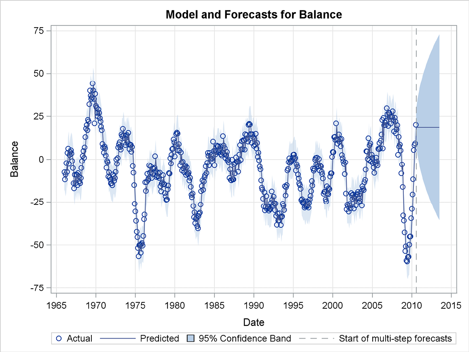
Figure 7.6 Forecast errors for exponential smoothing of the Swiss Business Indicator
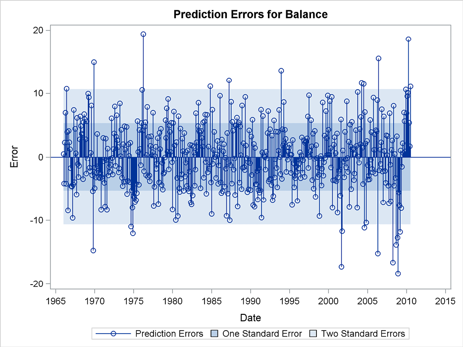
The forecast errors in the observation period are plotted as a part of the graphical output from the ESM procedure. (See Figure 7.6.) These errors indicate systematic behavior of the forecasts because the method mainly forecasts by replicating the latest observation. The data series has the form of a smooth curve. The long periods with a constant upward or downward tendency give the same sign of the forecast errors for many consecutive months. The autocorrelation plot of the forecast errors also shows that the forecasting procedure can be improved, because many autocorrelations are outside the confidence band. (See Figure 7.7.) Other plots in the output stress this point as well.
Notice, however, that the lag 12 autocorrelation for the forecasting errors corresponds to a yearly seasonal pattern for this monthly series. This is insignificant. The facilities for seasonal forecasting in PROC ESM are not useful for improving the forecasts, and the various methods to include trends in the forecasts are also considered irrelevant because the Business Indicator series is by definition limited to an interval. In Section 7.9, a stepwise autoregressive forecasting method is applied to this series by the PROC VARMAX time series procedure.
Figure 7.7 Autocorrelation function for the forecast errors

7.9 Fitting Models for the Swiss Business Indicator Using PROC VARMAX
In this section, PROC VARMAX (instead of PROC ESM) is used to produce forecasts of the Swiss Business Indicator. This procedure uses modern automatic model selection facilities for the STEPAR method and includes facilities for automatic selection of Box-Jenkins ARMA models.
If no model is specified, then by default the procedure estimates the parameters in all ARMA(p,q) models of order up to p = 5 and q = 5. The “best” model is then chosen by minimizing the information criterion as described in Section 7.3. In many situations, the list of potential models is too large, and some of the proposed models fail during the estimation, especially for both p > 0 and q > 0, because the parameter space could be ill conditioned. For this reason, only autoregressive models are considered in this section, and the codes are restricted to mimic the stepwise autoregressive fitting forecasting procedures of Section 7.3.
The application of PROC VARMAX in Program 7.4 produces forecasts by the best autoregressive model of order at most p = 10. The forecasts are plotted by ODS Graphics System, which is invoked by the ODS GRAPHICS statements. The plot option is specified so that both a plot of observed time series values ending with the forecasts and a plot of only forecasts for the period after the last observation are made. However, only forecasting plots are requested, and all other potential plots are disregarded.
Program 7.4 Fitting an ARMA model for the Swiss Business Indicator with PROC VARMAX
ods graphics;
PROC VARMAX data=sasts.swiss_business_indicator plot=forecasts(all);
id date interval=month;
model balance/method=ml print=roots minic=(type=sbc p=10 q=0);
output out=outfor lead=120;
run;
ods graphics off;
The indexing variable for the time is stated in the ID statement. In Program 7.4, the variable is named date. Even if no seasonal effects are specified in the model, it is good practice to state the interval option in order to ensure that horizontal axes in the plots are printed correctly.
The central statement is the MODEL statement where the variable to be forecast (balance) is specified and details for the selected algorithms are written. The option method=ml specifies that full maximum likelihood estimation of the parameters is applied as an alternative to least squares estimation. This estimation method is more time consuming, but using modern numerical algorithms, it has now become standard. The minic=(type=sbc p=10 q=0) option specifies that all possible orders p up to p = 10 have to be tested, and the best is chosen. This option also specifies with q = 0 that no moving average components are included in any of the proposed models. The best model out of the ten possible autoregressive models is determined by using Schwarz’s Bayesian Criterion (SBC). This criterion introduces a rather severe penalty for over parameterization, but other criteria are available. (See Section 7.3.) The option minic= is an abbreviation for MINimum Information Criterion.
The forecasts are printed in the output window, and they are also stored in a new data set named Outfor as specified by the option out=outfor in the OUTPUT statement. The OUTPUT statement is mandatory for forecasting, but specifying an output data set is optional. Also, to suppress the printed output, specify the noprint option. The forecasts are derived up to horizon of 120 by the option lead=120, which is also in the OUTPUT statement. This long horizon is of no practical use, but it is used here to study the long-term performance of the forecasting function.
The best model is the AR(7) model, because the information criterion attains the lowest value for p = 7. The criterion value is printed in the output (Output 7.4). As seen from the estimated parameters, the lag five and lag six parameters are insignificant, but the lag seven parameter is highly significant. Therefore, the best model is p = 7. In model building for this series, perhaps a model of order four would be preferred in order to reduce the number of estimated parameters. However, the inclusion of some insignificant parameters presents no problems when the estimation is only for forecasting purposes. The residual variance—the innovation variance—which forms the basis for the construction of confidence limits for the forecasts, is estimated as 22.05 by the maximum likelihood method, which is a more efficient estimator than the residual sum of squares.
Output 7.4 Details of the model identification done by PROC VARMAX

The plot of observations and forecasts is shown in Figure 7.8, and a more detailed plot of the forecasting period is in Figure 7.9. The forecasts continue the cycling performance of the series in the observation period but tend toward a constant level in a couple of years. The average value of the observed series ![]() = - 5.89 is in fact also estimated by the procedure, but it is not clearly seen in the output because the estimated model constant
= - 5.89 is in fact also estimated by the procedure, but it is not clearly seen in the output because the estimated model constant ![]() = - 0.44 is a parameter of an alternative parameterization so that
= - 0.44 is a parameter of an alternative parameterization so that
![]() .
.
Figure 7.8 Forecasting using an autoregressive model of high order
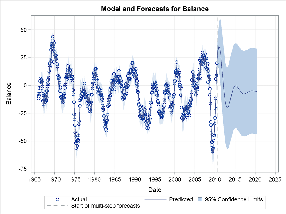
Figure 7.9 Forecasts of the Swiss Business Indicator with a cycle

For this series, it is obvious that forecasting a few months ahead is possible using the level of the most recent observations as the historical “good economic times” and also by assuming that these good times last for at least some months. Simple exponential smoothing as used in Section 7.8 extrapolates by a constant level close to the last observed value, which is reasonable for short-term forecasting. When predicting for a longer horizon, the past history is of limited importance because the history shows that good economic times seldom last for more than a couple of years. Forecasting for long horizons by the observed overall level of the observations seems intuitively reasonable because the Business Indicator index has a constant definition. The stepwise autoregressive method in this section combines these two views into a single forecasting procedure in a very convenient way.
In PROC VARMAX, the MODEL statement can include a linear or quadratic trend that is the long-run prediction. To include this trend, specify the option trend=linear or trend=quad in the MODEL statement. Similarly, seasonal dummies can be included by the option nseason=12.
Apart from being attractive as stated above, the forecasts of the fitted AR(7) model seem more interesting or even scientific because they are not simple horizontal or trending straight lines like the forecasts provided by the other forecasting methods. This difference is due to the behavior of forecasts in autoregressive models, which is a combination of damped exponentials and exponentially damped sinusoidal cycles. Studying the roots of the estimated autoregressive polynomial provides insight into the cycles’ behavior so that, for example, the wavelength of the business cycles can be derived. In Program 7.4, the code specifies that PROC VARMAX should write these roots in the output window by the print=roots option in the MODEL statement. See Box and Jenkins (1972) for a further, textbook-style exposition. The whole subject of business cycles for this series is treated by alternative methods in Section 10.3 on unobserved component models.
If the order of the autoregressive model is reduced to p = 4, the long-run forecast function after the first four predicted values is simply a mean looking reversion with no cycles; see Figure 7.10. This result is more boring, but when judged by the confidence limits, it seems just as possible as the more interesting cyclic form of the AR(7) forecasting function.
Figure 7.10 Forecasting the Swiss Business Indicator using an AR(4) model
